Selected Topics #1: Adversarial Attacks
Go back to Chapter 1: Digital Attack
Go back to Chapter 1: Prerequisites
Go back to Chapter 2: Physical Attack
Go back to Chapter 4: Countermeasure with Autoencoder Detection
Train a VGG16 white box model for the STL10 dataset
Contents
Introduction
As mentioned at the beginning, you are going to perform the white-box attacks, the attacks on physical level and the detection of adversarial images with an autoencoder based on the STL10 dataset. For that, you need to build a white-box model to be attacked.
Base
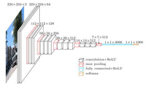
You can use different models as base models. In this tutorial you’re going to use the VGG16 model as base and fine-tune it for our purpose. The fine-tuning step first requires to load the VGG16 model without the top-layers, because you need to define them yourself to match the number of classes in the STL10 dataset. The architecture of the VGG16 model is shown below.

Fine tune
The fine-tune process starts after the last pooling layer by replacing the fully connected layers (blue layers in the chart). The feature extraction part remains. Since the pre-trained VGG model should be sufficient to classify the STL10 dataset, pay attention to set the weights of the feature extraction part to non-trainable.
The following layers should be sufficient for a good performance:
inputs = keras.Input(shape=(96,96,3))
x = base_model(x)
x = Flatten()(x)
x = Dense(1024, activation='relu')(x)
x = Dropout(0.4)(x)
pred = Dense(10, activation='softmax')(x)
The STL10 dataset includes images of the size $96x96x3$ and ten different classes. Therefore, the final output layers has ten neurons. Our suggestion is to set the dropout value pretty high to prevent the complex model to overfit on the training data.
Swap datasets
The original dataset contains 5000 training and 8000 test images. In order to increase the number of training data, you can swap these datasets. Keep in mind that by swapping these datasets, the comparability with public results for the dataset is lost, but this is okay, because we only need a accurate model to show the effectiveness of the attacks.
Prerequisites
Imports
Below are all of the modules that must be installed and imported to run this tutorial. You’re going to use the Keras library because it’s easier to understand.
import keras
from keras.models import Sequential, load_model
from keras.layers import Dense, Flatten, Conv2D, MaxPooling2D, Activation, Dropout
import numpy as np
from keras.datasets import cifar10
import os
import tensorflow as tf
from extra_keras_datasets import stl10
import keras.backend as k
from keras.applications.vgg16 import VGG16
from keras.engine import Model
from keras import optimizers
import matplotlib.pyplot as plt
import seaborn as sns
sns.set()

# Suppress tensorflow deprecation warnings
import tensorflow.python.util.deprecation as deprecation
deprecation._PRINT_DEPRECATION_WARNINGS = False
Using TensorFlow backend.
Define classes and get data
Define the class labels of the STL10 dataset and read in the data. Do some small preprocessing steps like converting the $y$ values to categorical ones and scale the $x$ between $0$ and $1$ .
# define class labels and number of classes
class_list = ["airplane", "bird", "car", "cat", "deer", "dog", "horse", "monkey", "ship", "truck"]
num_classes = 10

# define width, height and dimension of images
w, h, d = 96, 96, 3

# The data, split between train and test sets:
# SWAP datasets
(x_test, y_test), (x_train, y_train) = stl10.load_data()
print('x_train shape:', x_train.shape)
print(x_train.shape[0], 'train samples')
print(x_test.shape[0], 'test samples')

# Convert class vectors to binary class matrices.
# Stl10 datasets starts with class 1, not 0
y_train = keras.utils.to_categorical(y_train-1, num_classes)
y_test = keras.utils.to_categorical(y_test-1, num_classes)

# Scale data between 0 and 1
x_train = x_train.astype('float32')
x_test = x_test.astype('float32')
x_train /= 255
x_test /= 255
x_train shape: (8000, 96, 96, 3)
8000 train samples
5000 test samples
Fine Tune the Model
Use the Adam optimizer along with:
- a learning rate of $lr=0.001$ and
- a batch size of $128$ .
Train/Fine-tune the model for only $10$ epochs to avoid overfitting.
Helper functions
These methods build the layers on top of the VGG16 model and the interface to start the fine-tuning. Pay attention to set the layers of the base model to non-trainable.
def adapt_classifier(base_model, train_all_layers=False):
    """
    This method builds the model for the fine tuning process, based on the base_model
    :param base_model:         model we want to fine tune
    :param train_all_layers:   whether we only want to train the fully connected layers

    :return model:             compiled model architecture
    """

    # build architecture
    inputs = keras.Input(shape=(96,96,3))
    #x = keras.layers.UpSampling2D()(inputs)
    x = base_model(inputs)
    x = Flatten()(x)
    x = Dense(1024, activation='relu')(x)
    x = Dropout(0.4)(x)
    pred = Dense(10, activation='softmax')(x)

    #build model
    model = Model(inputs, pred)

    # set layers of base model to train_all_layers
    for layer in base_model.layers:
        layer.trainable = train_all_layers

    # compile with Adam and learning rate 0.001
    model.compile(loss='categorical_crossentropy',
                  optimizer=optimizers.Adam(lr=0.001),
                  metrics=['accuracy'])
    return model

def fine_tune(model, x_train, y_train, x_test, y_test, batch_size):
    """
    This method actually calls the fit method of the model we pass
    :param model:          model we want to train
    :param x_train:        train data x
    :param y_train:        train labels y
    :param x_test:         test/validation data
    :param y_test:         test/validation labels
    :param batch_size:     Batch size during training

    :return history:       train statistics
    """

    history = model.fit(x_train, y_train,
          batch_size=batch_size,
          epochs=10,
          validation_data=(x_test, y_test),
          shuffle=True)

    return history
Start fine-tuning
# build the model
model = adapt_classifier(VGG16(weights='imagenet', include_top=False, input_shape=(w, h, d)))
# get the training statistics
history = fine_tune(model, x_train, y_train, x_test, y_test, 128)
Save model in h5 format
Saving the model in the h5 format allows us to import it very easy with the load_model method from the Keras API.
# save model
save_dir = 'final_models'
model_name = 'vgg16_stl10.h5'
if not os.path.isdir(save_dir):
    os.makedirs(save_dir)
model_path = os.path.join(save_dir, model_name)
model.save(model_path)
Plot training and validation loss
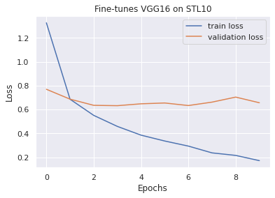
Below you can plot the training and validation loss to identify overfitting and to look at the stability of the training in general.
# define figure
plt.title("Fine-tunes VGG16 on STL10")
plt.plot(history.history["loss"], label="train loss")
plt.plot(history.history["val_loss"], label="validation loss")
plt.xlabel("Epochs")
plt.ylabel("Loss")
plt.legend()
plt.show()

Observation:The model overfits relatively quickly, even with a high dropout value. This could be due to the very good feature extractor of the VGG model and the rather small amount of training data. The classification task seems to be easy for the model to solve. But since the validation loss does not increase strongly, but rather remains constant, this model is okay for our needs.
Model accuracy on training and test data
The model achieves an accuracy of almost ~99 percent on the training data and ~79 percent on test data. Feel free to try out some other architectures in order to get better results on the test data.
print(f"Model accuracy on train data: {model.evaluate(x_train, y_train)[1]}")
print(f"Model accuracy on test test: {model.evaluate(x_test, y_test)[1]}")
8000/8000 [==============================] - 6s 796us/step
Model accuracy on train data: 0.9853749871253967

5000/5000 [==============================] - 4s 766us/step
Model accuracy on test test: 0.7874000072479248
Sources
[1] STL-10 dataset
[2] Very Deep Convolutional for large-scale image recognition
[3] Step by step VGG16 implementation in Keras for beginners
[4] Adam: A Method for Stochastic Optimization
