

Selected Topics #1: Adversarial Attacks
Chapter 1: Digital Attack
Contents
- Introduction
- Prerequisites
- Attack Classes
- Prepare for Creating Adversarial Images
- Using FGSM
- Using PGD
- Validation on Complete Test Dataset
- Conclusion
- Sources
Introduction
This first chapter deals with digital adversarial attacks, which can be implemented with the help of gradients. The gradient based attacks assume that an attacker is in possession of the model they want to attack. These attacks can therefore be classified as white-box attacks.
In this first chapter, the Fast Gradient Sign Method[1] is introduced. An extension of this method is the Projected Gradient Descent Method [2],[3],[4]. As you have read in the intro, there are of course many white-box attack methods. We’ve decided to focus on these two because you don’t need much previous knowledge to understand these methods, the PGD is based on FGSM and both can be evaluated quickly.
In the following, you’re going to learn the theory of the attacks, see the corresponding implementation and evaluate the attacks using the STL10 dataset.
White-Box Model
Every white-box attack needs a white-box model to be attacked. For that, you’re going to fine-tune a VGG16 model. Take a look here: Train a white box model.
Fast Gradient Sign Method (FGSM)
Generating adversarial examples with the Fast Gradient Sign Method was first introduced in the work Explaining and harnessing adversarial examples by Goodfellow et al. in 2014. First step, remember what gradients are.
What are gradients?
The gradient of a function $\nabla f$ in general is a fancy word for the derivative or the rate of change of a function $f$ . It’s a vector (a direction to move) that points in the direction of greatest increase of that function. Let’s take a function $f$ with $4$ variables. The gradient $\nabla_{x}$ can be built by computing the partial derivatives:
Machine Learning often includes an optimization problem that can be solved by minimizing a specific loss function $\mathcal{L}$ . A loss function tells us “how good” our model is at making predictions for a given set of parameters, by measuring the difference between the ground truth $\mathcal{y}$ and our model’s prediction $\mathcal{\hat y}$ , given an input $x$ . $\mathcal{L}$ has its own curve and its own gradients. The slope of this curve tells us how to update our parameters to make the model more accurate. During the training of a model, we can change the model parameters $\theta$ to minimize the loss function. Since we need to consider the impact each parameter has on the final prediction, the partial derivatives of the loss function $\mathcal{L}$ with respect to $\theta$ are calculated, that is the gradient $\nabla_{\theta} \mathcal{L}$ . Since the gradient points in the direction of the steepest rise, the parameters are updated in the direction of the negative gradient to minimize $\mathcal{L}$ :
\begin{equation*} \theta = \theta - n * \nabla_{\theta}\mathcal{L(\theta, x, y}) \end{equation*}$n$ is called the learning rate. This procedure is known as Gradient Descent [5].
What changes in case of adversarial attacks?
To what extent are gradients useful in the context of adversarial attacks? In the previous section we’ve shown you the equation to calculate the gradients with respect to the model parameters $\theta$ . You can’t optimize the parameters anymore because you’re not allowed to modify the model itself. The goal is instead to generate a certain input $x'$ that will steer the prediction of the model in a certain direction without changing the model. Thus, the gradient information is applied to the inputs instead of the model parameters. Like in the picture below, we want fool the model by adding a non-visible perturbation.
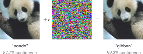
The model parameters should stay the same but what can be changed is the input itself, that is the pixel values in the images $x$ . The idea is to calculate the influence of each pixel value to the current model error. This can be done by computing the gradient $\nabla _x$ of $\mathcal{L}$ . The original images $x$ are manipulated by adding or subtracting a small noise $\epsilon$ to each pixel. Whether a noise is added or subtracted $\epsilon$ from a pixel value depends on the sign of the gradient. The result is called $x'$ . The difference between $x$ and $x'$ is the perturbation $\delta$ . Instead of using the true gradient values, we only consider the sign to maximize the effect of the perturbation.
As you have read in the intro, there are basically two different attack types: A targeted and an untargeted attack. Let’s have a closer look at the formula for updating the images in both cases:
Targeted Attack
For a targeted attack setting, the process can be seen as one step of the gradient descent method to solve the problem. In comparison to the regular procedure, where you would calculate the loss between the model’s prediction and the true value, the ground truth label is set to the label of our desired output class $T$ :
\begin{equation*} x' = x - \epsilon * sign(\nabla_{x}\mathcal{L(\theta, x, T})) \end{equation*}By adding noise in the direction of the negative gradient, you’re going to move the prediction of the model closer to the desired target class $T$ .
Untargeted Attack
For an untargeted attack, we don’t longer use the negative gradient, because the goal is now to increase the model error. We want to change the input image in a way that the model predicts any class, except the true class. Therefore the difference to the true class should be large.
\begin{equation*} x' = x + \epsilon * sign(\nabla_{x}\mathcal{L(\theta, x, y})) \end{equation*}By adding noise in the direction of the positive gradient, you’re going to move the prediction of the model away from the ground truth label.
One-step vs minimal perturbation?
We’re going to guide you through the implementation of two possible variants of this method. It’s important to mention that in both cases the gradient is calculated only once.
In case of the One-Step method, the calculated perturbation $\delta$ is added exactly one time to the image after multiplying it by $\epsilon$ . Since the amount of noise, which is necessary to fool the model varies from image to image, we also show you how to implement a Minimal-Step method. Here, the calculated perturbation is multiplied with a factor $\epsilon_{step}$ and added to the image. If the target is already reached, no further perturbation will be added to the image. If the attack is not yet successful, $\epsilon_{step}$ will be increased and the attack is repeated for the images where we do not yet have the desired output class.
Of course the perturbation should be as invisible as possible. To keep the size of $\delta$ controllable, you need to ensure that $|| \delta ||_\infty \leq \epsilon$ . This happens automatically in the One-Step method because $\delta * \epsilon$ is added in one step. In contrast, the Minimal-Step method will stop if the attack is successful on all input images or the constraint $|| \theta ||_\infty \leq \epsilon$ is violated. This becomes true as soon as $\epsilon_{step} > \epsilon$ .
Projected Gradient Descent (PGD)
Now you should have understood the basic principle of the FGSM method. It is fast because you only have to calculate the gradient once, but it should be clear that this is also a disadvantage. If you want to increase the amount of noise, you can only add the same perturbation again and again. Wouldn’t it be smarter to make the process iterative? This kind of process was used in works like Adversarial Machine Learning at Scale or Adversarial examples in the physical world.
The idea
You calculate a perturbation $\delta$ from the gradients, add it to the image and in the second step you calculate the gradients again, but on the already modified image from the previous step. This should give us a slightly different perturbation per step, so that we don’t stupidly add the same noise to the picture again and again.
As in the FGSM method, the size of the perturbation should be controllable. Therefore, $\epsilon$
and $\epsilon_{step}$
also exist in this attack method. During each iteration, we ensure that $|| \theta ||_\infty \leq \epsilon$
is not violated, by projecting $\delta$
into the norm ball. You can find more detail on the mathematical background of in the referenced paper Adversarial examples in the physical world. This projection can be achieved by simply clipping the values of $\delta$
to lie within the range $[-\epsilon,\epsilon]$
. There is no restriction on which norm to use, you can use any to calculate the norm ball. Have a look at the _projection method of the ProjectedGradientDescent class to see other examples than the simple value-clipping.
At first, this might seem similar to the FGSM minimal attack method, but the difference is that the algorithm does not stop if $\epsilon_{step} \gt \epsilon$ . Because we always calculate the new gradient and calculate a new perturbation, the noise can still change, even if $\epsilon_{step} \gt \epsilon$ .
Targeted Attack
Let’s say, you’re at the time step $t$ . You can then formulate the process for a targeted PGD attack with the following equation:
Subtract the perturbation, computed by building the gradients from the loss between the model’s prediction and the target class, from the image of the previous step and ensure that all values are in the valid range.
Untargeted Attack
And for an untargeted attack:
Add the perturbation, computed by building the gradients from the loss between the model’s prediction and the ground truth label, to the image of the previous step and ensure that all values are in the valid range.
Let’s take a look at how you can implement these attacks!
Prerequisites
Imports
Below are all of the modules that must be installed and imported to run this tutorial. You’re going to use the Keras interface, because it is easier to understand than tensorflow.
import keras
from keras.models import Sequential, load_model
from keras.layers import Dense, Flatten, Conv2D, MaxPooling2D, Activation, Dropout
import numpy as np
from keras.datasets import cifar10
import os
import tensorflow as tf
from extra_keras_datasets import stl10
import keras.backend as k
from keras.applications.vgg16 import VGG16
from keras.engine import Model
import matplotlib.pyplot as plt
import seaborn as sns
import time
from tqdm.notebook import trange
Using TensorFlow backend.
Define classes and get data of STL10
# define stl10 class list
class_list = ["airplane", "bird", "car", "cat", "deer", "dog", "horse", "monkey", "ship", "truck"]
num_classes = 10

# define width, height and dimension of images
w, h, d = 96, 96, 3

# The data, split between train and test sets:
(x_test, y_test), (x_train, y_train)= stl10.load_data()
print('x_train shape:', x_train.shape)
print(x_train.shape[0], 'train samples')
print(x_test.shape[0], 'test samples')

# Convert class vectors to binary class matrices.
# Stl10 datasets starts with class 1, not 0
y_train = keras.utils.to_categorical(y_train-1, num_classes)
y_test = keras.utils.to_categorical(y_test-1, num_classes)

# Scale data between 0 and 1
x_train = x_train.astype('float32')
x_test = x_test.astype('float32')
x_train /= 255
x_test /= 255
x_train shape: (8000, 96, 96, 3)
8000 train samples
5000 test samples
Load the white-box model
Have a look at Creating your white box model if you want to attack your own model.
model = load_model("./final_models/vgg16_stl10.h5")
print(f"Model accuracy on train data: {model.evaluate(x_train, y_train)[1]}")
print(f"Model accuracy on test test: {model.evaluate(x_test, y_test)[1]}")
8000/8000 [==============================] - 7s 870us/step
Model accuracy on train data: 0.9853749871253967

5000/5000 [==============================] - 4s 775us/step
Model accuracy on test test: 0.7874000072479248
Plot function
This function receives some images, lets the passed model predict on them and plots the images with their model prediction.
def plot_images(images, columns, rows, title, model, targets=None, gt=None, size=(15, 8)):

    """
    This function is used to plot images with their corresponding model prediction
    :param images:        some images
    :param columns:       cols of figure
    :param rows:          rows of figure
    :param title:         title of figure
    :param model:         model to predict the class labels
    :param target:        target lists
    :param gt:            ground truth labels
    """

    sns.set_style("whitegrid", {'axes.grid' : False})

    # create figre
    fig=plt.figure(figsize=size)
    plt.suptitle(title, fontsize=16)
    columns = columns
    rows = rows

    # for each image, let the model predict its class label
    for i in range(1, columns*rows +1):

        # let model predict
        img = images[i-1]
        fig.add_subplot(rows, columns, i)
        pred = model.predict(images[i-1].reshape(1, w, h, d))
        pred_class = class_list[np.argmax(pred.flatten())]
        pred_class_conf_prob = max(pred.flatten())

        # plot different things depending on the passed arguments
        if targets is not None:
            pred_target_class = max(pred.flatten()*targets[i-1])
            plt.title(f"{pred_class} ({pred_class_conf_prob:.2f})\nTarget: {pred_target_class:.2f}")
        elif gt is not None:
            plt.title(f"{pred_class} ({pred_class_conf_prob:.2f})\nG.T.: {gt[i-1]}")
        else:
            plt.title(f"{pred_class} ({pred_class_conf_prob:.2f})")

        plt.imshow(img)
    plt.show()


def plot_bar(eps, eps_step, n_steps, gt):
    """
    Generate a horizontal bar plot to show how often we had to add the noise
    in case of the minimal attack method
    :param eps:        maximum amount of noise
    :param eps_step:   noise per step
    :param n_steps:    results from attack
    :param gt:         gt label
    """
    sns.set()

    plt.title("Amount of noise added to the image")
    plt.ylabel("Initial Image")
    plt.xlabel("Number of steps")
    y_pos = np.arange(len(gt))

    # Create horizontal bars
    plt.barh(y_pos, n_steps)

    # Create names on the y-axis
    plt.yticks(y_pos, gt)
    plt.xlim(0, int(eps/eps_step))
    plt.xticks(np.arange(0, int(eps/eps_step)+1, 1))
    # Show graphic
    plt.show()
Attack Classes
Parent class
This is our base gradient attack class. The FGSM and the PGD inherit from this class. You can specify a range for clipping the final images. By default this is set to the range $[0, 1]$ because this is the valid float range for images. There are methods for building the tensorflow graph, computing the gradients and perturbation, applying the perturbation and clipping the noise values. Have a closer look at the implementation. We’ve commented all important parts.
class GradientAttack():
    """
    Base class for gradient attack. Builds graph of operations and defines function for calculating the gradient
    """


    def __init__(self, classifier, clip):
        """
        Initialize the class variables
        :parm classifier:    This is the model we want to attack
        :clip clip:          Range to clipp the final images
        """

        self.classifier = classifier
        self.clip_min = clip[0]
        self.clip_max = clip[1]

        # these variables can be set
        self.attack_params = ["norm", "eps", "eps_step", "targeted", "clip"]

        # build the attack graph once
        self._build()


    def set_params(self, **kwargs):
        """
        Handles updates of the class variables
        """
        for key, value in kwargs.items():
            if key in self.attack_params:
                setattr(self, key, value)
            else:
                raise KeyError("Unkown property ", key)
        return True


    def generate(self, x_org, targets):
        """
        This class needs to be implemented by the child classes
        :param x_org:   original images we want to add the pertubation
        :param targets: list of target classes
        """
        raise NotImplementedError()


    def _build(self):
        """
        Setup the attack graph
        """
        # placeholder for target vectors
        target_ph = k.placeholder(shape=self.classifier.output.shape)

        # loss function
        loss_function = k.categorical_crossentropy
        loss = loss_function(target_ph, self.classifier.output, from_logits=False)

        # calculate gradients with respect to the classifier's input
        loss_gradients = k.gradients(loss, self.classifier.input)[0]

        # function which expects the inputs and returns the gradients
        self._loss_gradients = k.function([self.classifier.input, target_ph], [loss, loss_gradients])


    def _get_loss_gradient(self, x, target):
        """
        This method calls the keras function for computing the gradients
        :param x:           input images
        :param target       target list

        :return gradients   gradients with respect to pixels
        """
        loss, gradients = self._loss_gradients([x, target])
        return gradients


    def _compute_perturbation(self, x_org, targets):
        """
        This method gets called in case of minimal attack method.
        We don't clip the pertubation at this point, but just return the sign of it
        :param x_org:     input images
        :param targets:   target of lists

        :returns sign of gradients
        """

        if self.targeted:
            grad = -self._get_loss_gradient(x_org, targets)
        else:
            grad = self._get_loss_gradient(x_org, targets)

        # Apply norm bound
        if self.norm == np.inf:
            grad = np.sign(grad)

        """
        There can be other norms to use on the gradients
        elif self.norm == 1:
            ind = tuple(range(1, len(x.shape)))
            grad = grad / (np.sum(np.abs(grad), axis=ind, keepdims=True) + tol)
        elif self.norm == 2:
            ind = tuple(range(1, len(x.shape)))
            grad = grad / (np.sqrt(np.sum(np.square(grad), axis=ind, keepdims=True)) + tol)
        """
        return grad


    def _apply_perturbation(self, x, perturbation, eps_step):
        """
        This method adds the pertubation multiplied with factor to the image and clips it to the defined range.
        In the one step attack, eps_step equals epsilon
        :param x:               input image
        :param perturbation:    noise
        :param eps_step:        factor to multiply the noise

        :return x:              modified input image with noise
        """

        x = x + eps_step * perturbation
        x = np.clip(x, self.clip_min , self.clip_max)

        return x


    def _compute_and_apply(self, x, x_init, targets, eps, eps_step):
        """
        This method combines the process of computing the perturbation and applying it to the image
        :param x:         variable we add noise
        :param x_init:    original image
        :param targets:   target list
        :param eps:       defines max amount of noise
        :param eps_step:  defines amount of noise we add per step

        :return adv_x:    the adverarial image
        """
        perturbation = self._compute_perturbation(x, targets)
        x = self._apply_perturbation(x, perturbation, eps_step)

        # here we calculate the differences between the adversarial images and the initial image
        # projection does the clipping
        perturbation = self._projection(x - x_init, eps)
        adv_x = x_init + perturbation

        return adv_x

    def _projection(self, values, eps):
        """
        This method does the clipping of epsilon values.
        In the simplest case the norm is np.inf, but there could be other norms.
        :param values: differences between x and x_init
        :param eps:    defines max amount of noise

        :returns      clipped pertubation
        """
        values_tmp = values.reshape((values.shape[0], -1))

        if self.norm == np.inf:
            # values_tmp contains the current noise. We first calculate the sign
            # and then taking the minimum of the current noise value and the maximum amount of
            # eps --> this is same like clipping the values
            values_tmp = np.sign(values_tmp) * np.minimum(abs(values_tmp), eps)

        """
        # other projection methods
        tol = 10e-8
        values_tmp = values.reshape((values.shape[0], -1))

        if self.norm == 2:
            values_tmp = values_tmp * np.expand_dims(
                np.minimum(1.0, eps / (np.linalg.norm(values_tmp, axis=1) + tol)), axis=1
            )
        elif self.norm == 1:
            values_tmp = values_tmp * np.expand_dims(
                np.minimum(1.0, eps / (np.linalg.norm(values_tmp, axis=1, ord=1) + tol)), axis=1
            )
        elif self.norm == np.inf:
            values_tmp = np.sign(values_tmp) * np.minimum(abs(values_tmp), eps)
        else:
            raise NotImplementedError("Values of `norm_p` different from 1, 2 and `np.inf` are currently not supported.")
        """

        values = values_tmp.reshape(values.shape)
        return values
First child class: Fast Gradient Sign Method Attack Class
This class implements the process of the FGSM attack.
It inherits all classes from the base class. There is also a function called _minimal_perturbation that implements the Minimal-Step attack method. The generate function is the starting point of the attack. Again the comments inside the class will guide you.
class FastGradientMethod(GradientAttack):
    """
    Implementation of fast gradient sign method
    """
    def __init__(self, classifier, clip=(0, 1), eps=0.3, norm=np.Inf, eps_step=0.01, targeted=False,
                 minimal=False):
        """
        Init all variables
        :param classifier:      white box model
        :param clip:            ranges to clip the adv images
        :param eps:             defines max amount of noise
        :param norm:            right now only np.inf: using sign and simple clipping
        :param eps_step:        how much noise we add per step
        :param targeted:        is the attack targeted or untargeted
        :param minimal:         do we want minimal attack method or one-step
        """

        # initialize the parent class
        super(FastGradientMethod, self).__init__(classifier, clip)

        # add additional class params, so that we can change them via set_params method
        self.attack_params += ["minimal"]
        kwargs = {
            "norm": norm,
            "eps": eps,
            "eps_step": eps_step,
            "targeted": targeted,
            "minimal": minimal
        }
        FastGradientMethod.set_params(self, **kwargs)


    def _minimal_perturbation(self, x_org, targets):
        """
        Method implements the minimal attack method. We stop adding noise to an image as soon as the attack is successfull.
        We stop the attack if all attacks are done or the maximum amount of noise is reached.
        :param x_org:     input images
        :param targets:   target list

        :return adv_x:    adversarial images
        :return n_steps:  Number of times the noise is added to the image
        """

        # make a copy of the initial image
        adv_x = x_org.copy()

        # calculate the pertubation ONCE!
        perturbation = self._compute_perturbation(x_org, targets)

        # initialize placeholders indicating which attack is already done
        active_indices = np.arange(x_org.shape[0])

        # save how much steps we needed per image
        n_steps = np.zeros(x_org.shape[0])

        # set current eps to the eps_step in the first iteration
        current_eps = self.eps_step

        # add noise if there are attacks left and current noise factor is below self.eps
        while active_indices.size > 0 and current_eps <= self.eps:

            # add perturabtion to the intial image
            current_x = self._apply_perturbation(x_org, perturbation, current_eps)

            # set adv images for all indices which are true (meaning the attack was not successfull)
            adv_x[active_indices] = current_x[active_indices]

            # increasing parameter for all active indices
            n_steps[active_indices] += 1

            # let the classifier predict
            adv_preds = self.classifier.predict(adv_x)

            # check for which images we've already have the desired output.
            if self.targeted:
                active_indices = np.where(np.argmax(targets, axis=1) != np.argmax(adv_preds, axis=1))[0]
            else:
                active_indices = np.where(np.argmax(targets, axis=1) == np.argmax(adv_preds, axis=1))[0]

            # increase the current step by adding eps_step
            current_eps += self.eps_step

        return adv_x, n_steps


    def generate(self, x_org, targets):
        """
        This method starts the attack
        :param x_org:     input images
        :param targets:   target lists
        """

        # call the corresponding functions for minimal attack and one-step attack
        if self.minimal:
            adv_x, n_steps = self._minimal_perturbation(x_org, targets)
            return adv_x, n_steps

        else:
            adv_x = self._compute_and_apply(x_org.copy(), x_org, targets, self.eps, self.eps)
            return adv_x
Second child class: Projected Gradient Descent Attack Class
This class implements the process of the PGD attack.
It inherits all classes from the base class. The generate function is the starting point of the attack. Again the comments inside the class will guide you.
class ProjectedGradientDescent(GradientAttack):
    """
    Class implements the projected gradient descent attack
    """
    def __init__(self, classifier, clip=(0, 1), eps=0.3, norm=np.Inf, eps_step=0.01, targeted=False,
                 max_iter=20):
        """
        Init all variables
        :param classifier:      white box model
        :param clip:            ranges to clip the adv images
        :param eps:             defines max amount of noise
        :param norm:            right now only np.inf: using sign and simple clipping
        :param eps_step:        how much noise we add per step
        :param targeted:        is the attack targeted or untargeted
        :param max_iter:        number of iteration equals to how often do we calculate gradients
        """

        # init parent
        super(ProjectedGradientDescent, self).__init__(classifier, clip)

        # adding class dependent variables
        self.attack_params += ["max_iter"]
        kwargs = {
            "norm": norm,
            "eps": eps,
            "eps_step": eps_step,
            "targeted": targeted,
            "max_iter": max_iter
        }
        ProjectedGradientDescent.set_params(self, **kwargs)


    def generate(self, x_org, targets, verbose=True):
        """
        Method starts the attack
        :param x_org:   input images
        :param targets: target list

        :return adv_x:  adv images
        """
        # make a copy
        adv_x = x_org.copy()

        if verbose:
            # do attack for max_iter iteration with trange
            for _ in trange(self.max_iter):
                adv_x = self._compute_and_apply(x=adv_x, x_init=x_org, targets=targets, eps=self.eps, eps_step=self.eps_step)
        else:
            # do attack for max_iter iteration with normal range
            for _ in range(self.max_iter):
                adv_x = self._compute_and_apply(x=adv_x, x_init=x_org, targets=targets, eps=self.eps, eps_step=self.eps_step)

        return adv_x
Prepare for Creating Adversarial Images
You already have loaded the STL10 dataset, your white-box model and have defined some plot functions. There are some steps left in order to start attacking the white-box model.
Get 10 example images from the test set
Search an image for each class where the model is pretty confident (>95 percent) that the class belongs to the true label. You’re going to use these images to investigate the effects of the attacks.
def get_example_from_each_class(x_test, y_test, confidence=0.8):
    """
    This method searches an example image for each class where the confidence of a model i above 80%
    """
    # list containing the example images
    images_for_adv = []
    # list containing the labels for the example images
    y_for_adv = []

    # let the model predict all test data
    test_softmax = model.predict(x_test)
    test_classes = np.argmax(test_softmax, axis=1)

    # search image for each class
    for class_idx in range(10):

        for i, y in enumerate(y_test):
            # get true label and models predictions
            true_label = np.argmax(y)
            pred = test_classes[i]
            pred_conf = test_softmax[i]
            # check if image is valid example
            if true_label==class_idx and true_label==pred and pred_conf[true_label]>confidence:
                images_for_adv.append(x_test[i])
                y_for_adv.append(y_test[i])
                break
    print("Example images found: ", len(images_for_adv))
    return images_for_adv, y_for_adv
images_for_adv, y_for_adv = get_example_from_each_class(x_test, y_test, confidence=0.95)
Example images found: 10
Plot image representations for each class
Call the plot function for each image.
plot_images(images_for_adv, 5, 2, "Selected images to demonstrate attack", model=model, targets=None, gt=[class_list[np.argmax(x)] for x in y_for_adv])

See how the model is pretty sure that the images belong to their true class? This is perfect for us, because we want attack the model on images, where it is confident.
Save images for physical attack
If you want to save these images for a later usage in the physical attack tutorial or detector tutorial, comment out the next cell
for i, img in enumerate(images_for_adv):
    plt.imsave(f"./physical_attack_data/imgs_gui/{class_list[i]}.jpg", img)

for i, img in enumerate(images_for_adv):
    plt.imsave(f"./detector_data/imgs/org/{class_list[i]}.jpg", img)
Labels for untargeted attack
For an untargeted attack, the labels correspond to their true labels.
x = np.array(images_for_adv)
y_untargeted = np.array(y_for_adv)
print(y_untargeted)
[[1. 0. 0. 0. 0. 0. 0. 0. 0. 0.]
 [0. 1. 0. 0. 0. 0. 0. 0. 0. 0.]
 [0. 0. 1. 0. 0. 0. 0. 0. 0. 0.]
 [0. 0. 0. 1. 0. 0. 0. 0. 0. 0.]
 [0. 0. 0. 0. 1. 0. 0. 0. 0. 0.]
 [0. 0. 0. 0. 0. 1. 0. 0. 0. 0.]
 [0. 0. 0. 0. 0. 0. 1. 0. 0. 0.]
 [0. 0. 0. 0. 0. 0. 0. 1. 0. 0.]
 [0. 0. 0. 0. 0. 0. 0. 0. 1. 0.]
 [0. 0. 0. 0. 0. 0. 0. 0. 0. 1.]]
Labels for targeted attack
You can select any target class you want. We just give you a suggestion. For a targeted attack, we’ve decided to set a technical target for all non-technical images and vice versa. Therefore, the goal is to fool the model to predict the class horse for all technical images and the class airplane for all non technical images:
- bird, cat, deer, dog, horse and monkey should be classified as airplane
- airplane, car, ship and truck should be classified as horse
target_list = [class_list.index("horse") if i in [0, 2, 8, 9]
               else class_list.index("airplane") for i in np.argmax(y_untargeted, axis=1)]
y_targeted = keras.utils.to_categorical(target_list, 10)
print(y_targeted)
[[0. 0. 0. 0. 0. 0. 1. 0. 0. 0.]
 [1. 0. 0. 0. 0. 0. 0. 0. 0. 0.]
 [0. 0. 0. 0. 0. 0. 1. 0. 0. 0.]
 [1. 0. 0. 0. 0. 0. 0. 0. 0. 0.]
 [1. 0. 0. 0. 0. 0. 0. 0. 0. 0.]
 [1. 0. 0. 0. 0. 0. 0. 0. 0. 0.]
 [1. 0. 0. 0. 0. 0. 0. 0. 0. 0.]
 [1. 0. 0. 0. 0. 0. 0. 0. 0. 0.]
 [0. 0. 0. 0. 0. 0. 1. 0. 0. 0.]
 [0. 0. 0. 0. 0. 0. 1. 0. 0. 0.]]
Now we finally get to the exciting part!
Using FGSM
Untargeted Attack
Let’s start with an untargeted FGSM attack by first instantiating the attack class.
# instantiate class
fgm_attack = FastGradientMethod(classifier=model, minimal=True, eps_step=0.001, eps=0.01, targeted=False)
Minimal-Step method
Settings:
- targeted = false
- $\epsilon_{step}$ = 0.001
- $\epsilon$ = 0.01
The maximum number of times that noise can be added to the image is ten.
adv_x, n_steps = fgm_attack.generate(x_org=x, targets=y_untargeted)
plot_images(adv_x, 5, 2, title="FGSM: Untargeted, Minimal Method", model=model, gt=[class_list[np.argmax(x)] for x in y_for_adv])
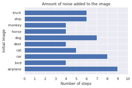
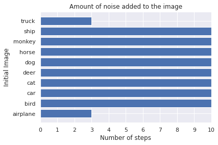
plot_bar(fgm_attack.eps, fgm_attack.eps_step, n_steps, gt=[class_list[np.argmax(x)] for x in y_for_adv])
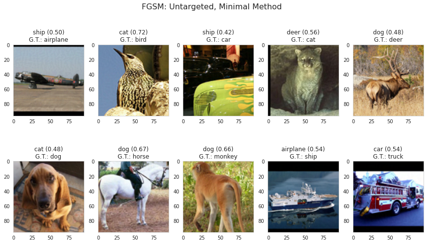
Observations:
- See how successful the attack is? The model always predicts a wrong label.
- The noise is almost not visible.
- A different amount of noise is necessary for the attack to be successful. The perturbation is added nine times on the airplane, but only four times on the monkey, horse, deer and bird.
- By making an untargeted attack, you are moving the prediction to the class that is closest to the current boundary. Therefore, the model predicts an animal class for all animals and a technical class for the the airplane, car, ship and truck.
One-step method
Remove the iterative process of increasing the noise and directly add a fixed amount of noise to the image. From the plot above you can see that with $\epsilon_{step}=0.006$ the attack is already successful, except for the classes airplane, car and dog. So if you just add the perturbation with the factor $\epsilon = 0.006$ to the picture, the attack should only work for the other classes.
Settings:
- targeted = false
- $\epsilon$ = 0.006
fgm_attack.set_params(minimal=False, eps=0.006)
adv_x = fgm_attack.generate(x_org=x, targets=y_untargeted)
plot_images(adv_x, 5, 2, title="FGSM: Untargeted, One-Step Method", model=model, gt=[class_list[np.argmax(x)] for x in y_for_adv])
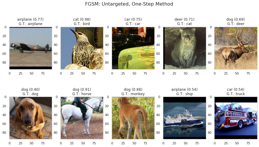
Observations:
As expected, the attack is only successful for the pictures, where the noise is added to the image up to 6 times in the first experiment.
Targeted attack
Minimal-Step method
Because we expect the targeted attack to be more difficult, increase the parameters.
Settings:
- targeted = true
- $\epsilon$ = 0.1
- $\epsilon_{step}$ = 0.01
fgm_attack.set_params(minimal=True, eps=0.1, eps_step=0.01, targeted=True)
adv_x, n_steps = fgm_attack.generate(x_org=x, targets=y_targeted)
plot_images(adv_x, 5, 2, title="FGSM: Targeted, Minimal Method", model=model, targets=y_targeted)
plot_bar(fgm_attack.eps, fgm_attack.eps_step, n_steps, gt=[class_list[np.argmax(x)] for x in y_for_adv])
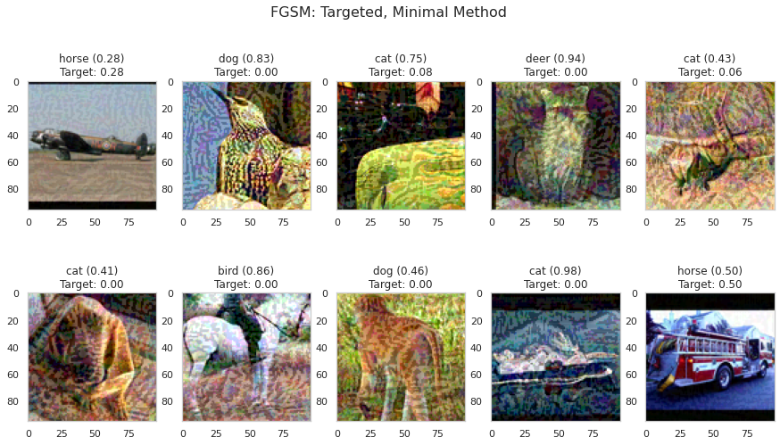
Observations:
The attack is only successful for two images. The truck and the airplane are classified as horse. The prediction of the other images does not correspond to our target class, but at least not to the true label.
Let’s see how successful the One-Step targeted attack is going to be.
One-step method
Settings:
- targeted = true
- $\epsilon$ = 0.1
fgm_attack.set_params(minimal=False, eps=0.1, targeted=True)
adv_x = fgm_attack.generate(x_org=x, targets=y_targeted)
plot_images(adv_x, 5, 2, title="FGSM: Targeted, One-Step Method", model=model, targets=y_targeted)

Observations:
- Only the attack on the truck is successful.
- Previously, the attack on the airplane has also worked. But by adding a fixed amount of noise on all pictures, that target class isn’t reached anymore. This shows that with this kind of attack, more perturbation is not always helpful because the perturbation is calculated only one time. So far, you don’t calculate a perturbation on already modified images.
Using PGD
Let’s see if the PGD method performs better than the FGSM. For comparability, use the same parameters like above.
# instantiate class
pgd_attack = ProjectedGradientDescent(model, max_iter=10, eps_step=0.001, eps=0.01, targeted=False)
Untargeted
Settings:
- targeted = false
- $\epsilon$ = 0.01
- $\epsilon_{step}$ = 0.001
- max_iter = 10
adv_x = pgd_attack.generate(x_org=x, targets=y_untargeted)
plot_images(adv_x, 5, 2, title="PGD: Untargeted", model=model, gt=[class_list[np.argmax(x)] for x in y_for_adv])

Observations:
The untargeted attack is successful without any visible noise. Again, technical objects are classified as other technical objects. Same for animals. This is also interesting, because you can find out which classes the model considers to be similar.
Targeted
Remember, the FGSM attack was only successful in two images with these settings:
- targeted = true
- $\epsilon$ = 0.1
- $\epsilon_{step}$ = 0.01
- max_iter = 40
pgd_attack.set_params(max_iter=40, eps=0.1, eps_step=0.01, targeted=True)
adv_x = pgd_attack.generate(x_org=x, targets=y_targeted)
plot_images(adv_x, 5, 2, title="PGD: Targeted", model=model, targets=y_targeted)
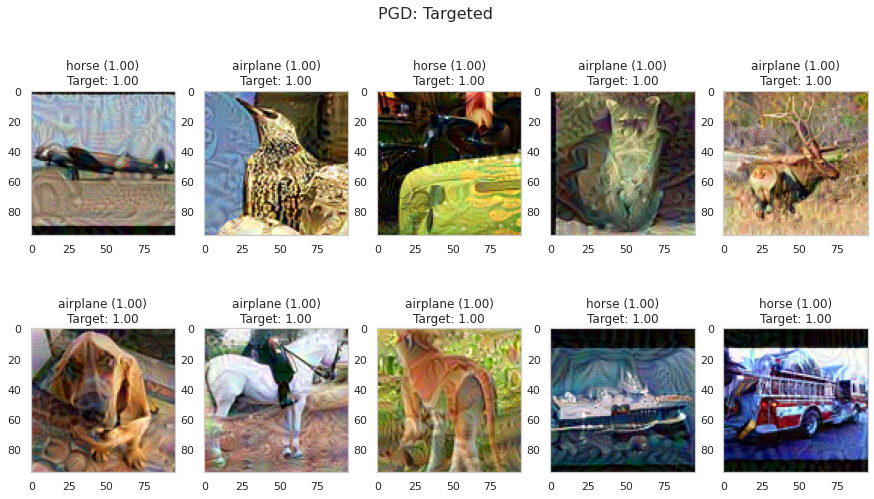
Observations:
Wow, that’s cool! The attack is successful for every single image. But the noise is highly visible. Can we improve this?
Targeted: Decrease epsilon
Decrease $\epsilon$ from $0.1$ to $0.03$ and $\epsilon_{step}$ from $0.01$ to $0.001$ . So the parameters are:
- targeted = true
- $\epsilon$ = 0.03
- $\epsilon_{step}$ = 0.001
- max_iter = 40
pgd_attack.set_params(max_iter=40, eps=0.03, eps_step=0.001, targeted=True)
adv_x = pgd_attack.generate(x_org=x, targets=y_targeted)
plot_images(adv_x, 5, 2, title="PGD: Targeted", model=model, targets=y_targeted)

Observations: Awesome! Without any highly visible noise, any technical object is classified as a horse with a confidence of $100$ %. In addition, all animals are classified as airplanes! Another point to mentioned is that unlike the FGSM, you can make any PGD attack work if you just add enough noise (increase epsilon).
Plot the noise
Let’s take the results from the last attack and plot the noise. Subtract the adversarial images from the original images and scale the differences between $0$ and $1$ by extracting the minimum and maximum value of all noise-images. This gives you the noise in a valid image range.
noise = np.abs(x-adv_x)
max_n = max(noise.flatten())
min_n = min(noise.flatten())
noise = (noise-min_n)/(max_n-min_n)
plot_images(noise, 5, 2, title="Noise", model=model, size=(15, 7))
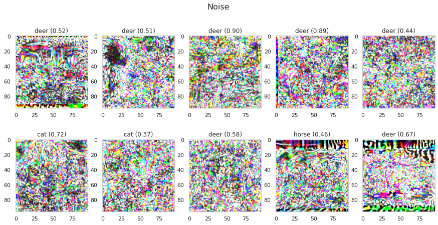
Observations:
- There are clear differences between the amount of noise in different regions.
- In black image regions like the borders, a lot of positive noise can be added because the pixels are zero. We can not add much positive noise to white pixels because all values that are greater than one are clipped to ensure a valid image space. Only negative noise can have an effect here.
- It’s also interesting that most of the noise is classified as deer.
Save attack images for detector example
For further usage you can save the images.
for i, img in enumerate(adv_x):
    plt.imsave(f"./detector_data/imgs/attack/{class_list[i]}.jpg", img)
Validation on Complete Test Dataset
To be able to make a more scientific statement about the performance of the attacks, you can now test the attacks on all 5000 test images of the STL10 dataset. With the current implementation, we’re not able to feed the whole test dataset at once. Therefore, split it up in packages of 500 and also measure the required computation time for creating the 5000 attack images. For our settings, we’ve summarized the results at the end of this chapter.
Untargeted attack
First, do an untargeted attack on the 5000 images. Set $\epsilon = 0.01$ for both methods.
FGSM
- targeted = false
- $\epsilon$ = 0.01
# fgsm untargeted on all test images
# instantiate class
fgm_attack = FastGradientMethod(model, eps=0.01, minimal=False, targeted=False)

adv_all_fgm_untargeted = []
start = time.time()

for i in trange(0, (len(x_test)-500)+1, 500):
    adv_x = fgm_attack.generate(x_org=x_test[i:i+500], targets=y_test[i:i+500])
    adv_all_fgm_untargeted.append(adv_x)

print(f"Attack done in: {time.time()-start:.2f}  seconds.")
adv_all_fgm_untargeted = np.array(adv_all_fgm_untargeted).reshape(-1, w, h, d)
print(f"Success rate of the attack: {1- model.evaluate(adv_all_fgm_untargeted, y_test)[1]}")
Attack done in: 7.67  seconds.
5000/5000 [==============================] - 3s 551us/step
Success rate of the attack: 0.847000002861023
# plot some results
idx = np.random.randint(0, len(adv_all_fgm_untargeted)-10)
plot_images(adv_all_fgm_untargeted[idx:idx+10], 5, 2, title="Example FGSM Untargeted ", model=model, size=(14, 6))
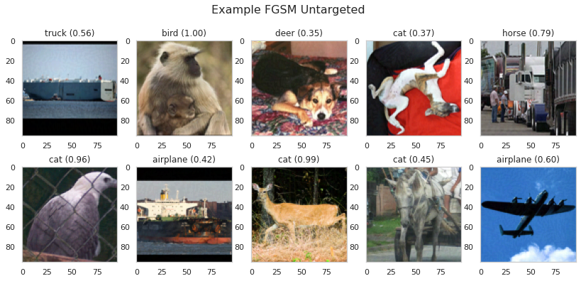
Observations:
The attack is successful in 84 percent of all input samples.
PGD
- targeted = false
- $\epsilon$ = 0.01
- $\epsilon_{step}$ = 0.001
- max_iter = 10
# pgd untargeted on all test images
# instantiate class
pgd_attack = ProjectedGradientDescent(model, max_iter=10, eps=0.01, eps_step=0.001)

adv_all_pgd_untargeted = []
start = time.time()

for i in trange(0, (len(x_test)-500)+1, 500):
    adv_x = pgd_attack.generate(x_org=x_test[i:i+500], targets=y_test[i:i+500], verbose=False)
    adv_all_pgd_untargeted.append(adv_x)

print(f"Attack done in: {time.time()-start:.2f}  seconds.")
adv_all_pgd_untargeted = np.array(adv_all_pgd_untargeted).reshape(-1, w, h, d)
print(f"Success rate of the attack: {1- model.evaluate(adv_all_pgd_untargeted, y_test)[1]}")
Attack done in: 72.87  seconds.
5000/5000 [==============================] - 3s 563us/step
Success rate of the attack: 0.9219999983906746
# plot some results
idx = np.random.randint(0, len(adv_all_pgd_untargeted)-10)
plot_images(adv_all_pgd_untargeted[idx:idx+10], 5, 2, title="Example PGD Untargeted ", model=model, size=(14, 6))
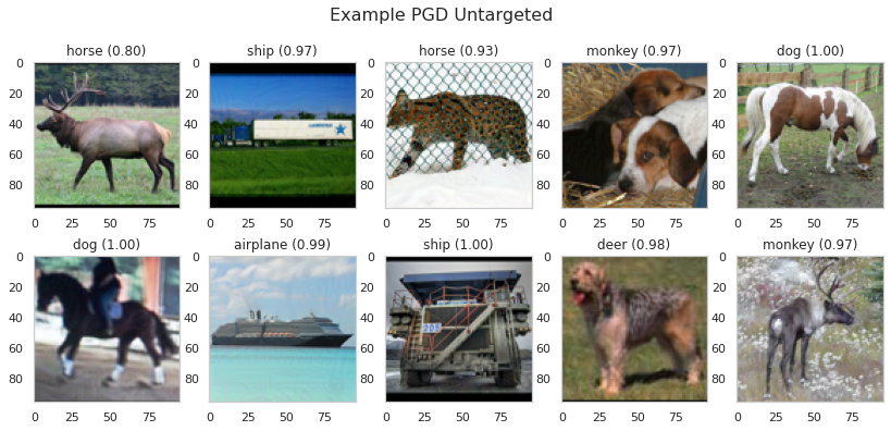
Observations:
In 92 percent of the samples, the attack is successful. That is almost 10 percent better than FGSM.
Now let’s create a targeted attack.
Targeted
Set $\epsilon = 0.03$ for both methods. A attack is only considered to be successful if the model predicts the target class. If the model predicts anything but the ground truth, this is will not count as success.
First iterate over the test labels and store our target label for each image
print(y_test.shape)
(5000, 10)
# assing every image with g.t. of 0, 2, 8, 9 the class horse
adv_targets = []
class_should_be_horse = [0, 2, 8, 9]

for y in y_test:
    dummy_label = np.zeros((1, 10))
    if np.argmax(y) in class_should_be_horse:
        dummy_label[0, class_list.index("horse")] = 1
        adv_targets.append(dummy_label)
    else:
        dummy_label[0, class_list.index("airplane")] = 1
        adv_targets.append(dummy_label)

adv_targets = np.array(adv_targets).reshape(-1, num_classes)
print(adv_targets.shape)
(5000, 10)
Now, create the attack images.
FGSM
- targeted = true
- $\epsilon$ = 0.03
# fgsm targeted on all test images
# instantiate class
fgm_attack = FastGradientMethod(model, eps=0.03, minimal=False, targeted=True)
adv_all_fgm = []
start = time.time()

for i in trange(0, (len(x_test)-500)+1, 500):
    adv_x = fgm_attack.generate(x_org=x_test[i:i+500], targets=adv_targets[i:i+500])
    adv_all_fgm.append(adv_x)

print(f"Attack done in: {time.time()-start:.2f}  seconds.")
adv_all_fgm = np.array(adv_all_fgm).reshape(-1, w, h, d)
print(f"Success rate of the attack: {model.evaluate(adv_all_fgm, adv_targets)[1]}")
Attack done in: 8.13  seconds.
5000/5000 [==============================] - 3s 561us/step
Success rate of the attack: 0.2924000024795532
#plot some examples
idx = np.random.randint(0, len(adv_all_fgm)-10)
plot_images(adv_all_fgm[idx:idx+10], 5, 2, title="Example FGSM Targeted ", model=model, size=(14, 8), targets=adv_targets[idx:idx+10])
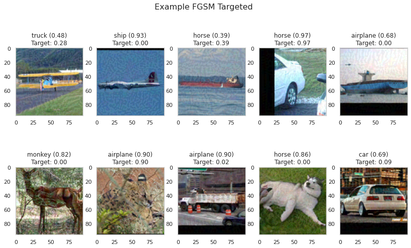
Observations:
In only 30 percent of the images, the attack was successful. But as you can see from the images above, most of the pictures have at least not the ground truth as a prediction.
Let’s see how the PGD method performs.
PGD
- targeted = true
- $\epsilon$ = 0.03
- $\epsilon_{step}$ = 0.001
- max_iter = 40
# pgd targeted on all test images. THIS TAKES SOME TIME
# instantiate class
pgd_attack = ProjectedGradientDescent(model, max_iter=40, eps=0.03, eps_step=0.001, targeted=True)

adv_all_pgd = []
start = time.time()

for i in trange(0, (len(x_test)-500)+1, 500):
    adv_x = pgd_attack.generate(x_org=x_test[i:i+500], targets=adv_targets[i:i+500], verbose=False)
    adv_all_pgd.append(adv_x)

print(f"Attack done in: {time.time()-start:.2f}  seconds.")
adv_all_pgd = np.array(adv_all_pgd).reshape(-1, w, h, d)
print(f"Success rate of the attack: {model.evaluate(adv_all_pgd, adv_targets)[1]}")
Attack done in: 287.41  seconds.
5000/5000 [==============================] - 3s 562us/step
Success rate of the attack: 0.9959999918937683
#plot some examples
idx = np.random.randint(0, len(adv_all_pgd)-10)
plot_images(adv_all_pgd[idx:idx+10], 5, 2, title="Example PGD Targeted ", model=model, size=(14, 8), targets=adv_targets[idx:idx+10])
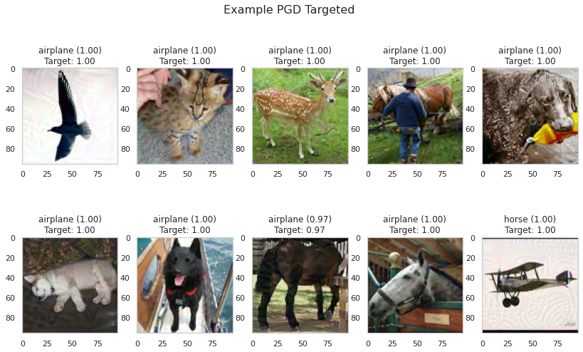
Observations:
That is impressive: 99.6 percent! It takes some time, but the attack is successful on almost every single image! The noise is seen in some images. Why don’t you try to reduce the noise even further.
Conclusion
This notebook should have given you an understanding of how to create adversarial images using gradient-based methods on a known model. Let’s summarize some observations:
On targeted and untargeted attacks
- In the case of untargeted attacks, a noise is generated that leads to a prediction of similar classes. Cars are classified as trucks, deer as dogs. This makes sense because the classes probably share some features and therefore the effort to move the prediction over the class boundary is likely low.
- FGSM already works quite well for the untargeted attack and is also very fast. In case of the targeted attack it doesn’t work that well. We are sure that this is the consequence of calculating the perturbation only once at the beginning and not again on already modified images. This is also the reason why more noise does not always lead to better results in this case.
- The PGD attack works well in both cases. Here, the assumption is correct that more noise leads to better results. But with the presented experiments it is shown that the targeted attack works well even with little noise.
Summary of the validation
The validation was done on 5000 test images of the STL10 dataset.
| Attack Method | Attack Type | Success rate (%) | Duration (s) |
|---|---|---|---|
| FGSM (one-step) | untargeted | 84.7 | 7.7 |
| PGD (max_iter=10) | untargeted | 92.1 | 72.8 |
| FGSM (one-step) | targeted | 29.2 | 8.1 |
| PGD (max_iter=40) | targeted | 99.5 | 287.5 |
We clearly see the best results using the PGD method. But because of the iterative process and due to the multiple calculations of the gradient, the attack is clearly slower than the FGSM method. In case of an untargeted attack the FGSM method is not much worse than the PGD. The situation is different with the targeted attack.
Where to Look Next
- You could look for another dataset or another white-box model and validate the attacks on them. We have also tried the attacks on different ResNet architectures and have achieved similar results.
- Of course, there are far more white-box attacks than the gradient based ones. In the introduction we have linked some very interesting papers, in case you are interested in looking at more attack techniques. Classic white-box attacks are rather untypical in reality, because in security critical areas you rarely have access to the complete model.
- Look at the next chapter, which is on physical attacks!
Sources
[1] Explaining and harnessing adversarial examples
[2] Adversarial Machine Learning at Scale
[3] Adversarial examples in the physical world
[4] Towards Deep Learning Models Resistant to Adversarial Attacks
[5] Deep Learning, S.82-86