

Selected Topics #1: Adversarial Attacks
Chapter 2: Physical Attack
Contents
- Introduction
- Prerequisites
- Physical Attack Class
- Define GUI with Jupyter Widgets
- Run Attacks
- Validate Different Masks on 2000 Test Images
- Let us Put the Attack on a Physical Level
- Conclusion
- Sources
Introduction
You should now have understood how to generate adversarial images using the FGSM and PGD methods. These images can deceive a model in the digital domain, but they are not directly transferable to the physical world.
Why? Because with the methods presented so far, you have created perturbation without limiting it to a certain image area. In addition, you’ve created the perturbation without paying attention to the printability of colors. How can you create a perturbation that is limited to a certain area and may only contain printable or inconspicuous colors?
There are some very interesting works on this topic, which we have used as a base for this tutorial:
- Robust Physical-World Attacks on Deep Learning Models [1] is about fooling a traffic sign detection model by generating stickers and putting them on the signs.
- Real and Stealthy Attacks on State-of-the-Art Face Recognition [2] is about fooling a face recognition system by generating noise in form of ‘glasses’. They show that by wearing this printed ‘glasses’ they can lead the prediction of the model to a famous actor/actress.
How does it work in general?
Compared to the FGSM and PGD method, we don’t need to calculate the gradient on the pixels in the input. It is simpler. We’re going to define our perturbation $\delta$ as a variable, whose values are optimized by an optimizer, e.g. Adam [3]. Before the optimizer can change the elements in $\delta$ , we’re going to mask certain areas of $\delta$ by multiplying it with a mask $\mathcal{m}$ . Therefore, the perturbation only affects specific areas of the image. You need to follow these steps:
- Initialize a variable $\delta$ with random values and load an input image $img$
- Multiply $\delta$ with a mask $\mathcal{m}$ that only contains areas with ones and zeros. The ones in the mask indicate the changeable elements in $\delta$ : $ \mathcal{m}* \delta$
- Compute the inverse of the mask and multiply it with the current image: $(1 - \mathcal{m}) * img$
- Add the masked image to the masked perturbation: $[\mathcal{m}* \delta] + [(1 - \mathcal{m}) * img]$
- Feed the image to the classification network and get the prediction
- Calculate the loss $\mathcal{L}$
- Use Gradient Descent[4] with an optimizer like Adam to change the elements of the noise to minimize $\mathcal{L}$
- Return to step 2 or stop the training if the number of epochs are reached
These steps can be visualized as followed:
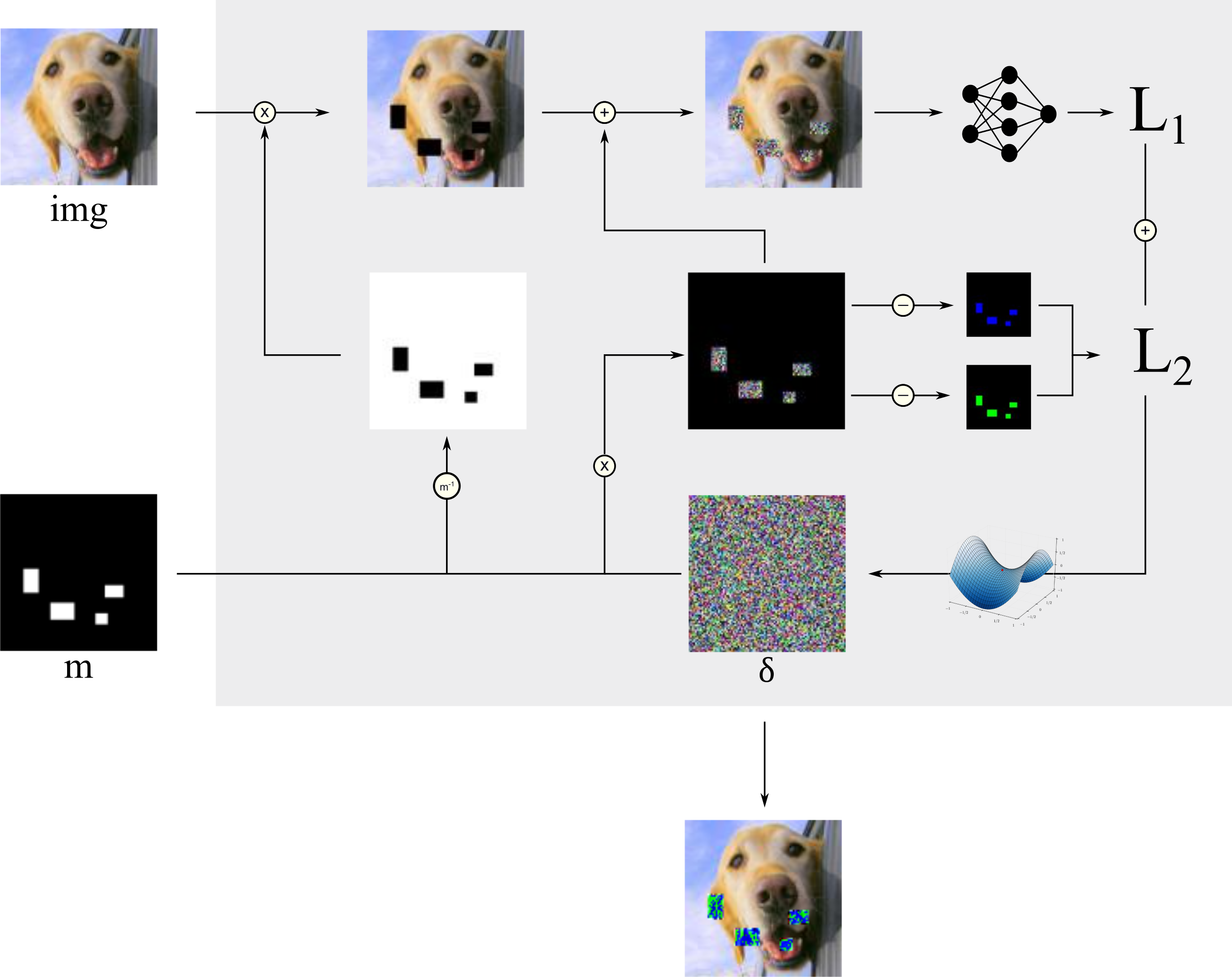
The loss $\mathcal{L}$
As you can see from the image above, there is $\mathcal{L}_1$ and $\mathcal{L}_2$ :
$\mathcal{L}_1$ : Of course the loss includes how good the model is in predicting our desired target class. This can be achieved by simply calculating the crossentropy between our target and the model’s prediction. Again, you have to distinguish between a targeted and an untargeted attack.
- In a targeted attack, the “ground truth” label, that is passed to the loss function, is the desired target $T$ . If the loss is small, the model will predict the target class:
- In an untargeted attack, pass the true ground truth label to the loss function. Therefore, a small loss indicates that the model makes the correct prediction. Because we want the model to predict anything but the true class, you need compute the inverse of the crossentropy value. To avoid division by zero, add a small number $\gamma$ to the denominator:
$\mathcal{L}_2$ : Moreover, the loss is influences by an error that is called printer error. Before the attack starts, the user can specify some colors, he prefers to have in the perturbation. The reason for that might be to ensure good printability or to have unobtrusive colors in $\delta$ . The printer error measures how close each pixel value is to these colors. For this, the defined colors are used to create monochrome images with the same dimension as the input image. $\mathcal{L}_2$ will be small, if each pixel value is close to one of the pre-defined colors. See the pseudocode below to understand how $\mathcal{L}_2$ is calculated:
pixel_element_diff = squared_difference(masked_noise, printable_colors*mask)
pixel_diff = reduce_sum(pixel_element_diff, 3)
reduce_prod = reduce_prod(pixel_diff, 0)
printer_error = reduce_sum(reduce_prod)
Another part you could include in the loss is the amount of the noise itself. You could use some kind of regularization to penalize big values in the perturbation. We dispense this part because it is not important for us to limit the amount of noise we produce in $\delta$ .
In order to control the influence of the printer error, the printer error is weighted with $\lambda_{printer}$ :
\begin{equation*} \mathcal{L} = \mathcal{L_1} + \lambda_{printer} *\mathcal{L_2} \end{equation*}What is not shown in this tutorial
Missing extraction from backgrounds
In this tutorial we have omitted 2 things to keep it simple. We’ve defined masks which have the same size as our input images: $96x96x3$ . In a realistic environment, we would first have to separate the background from the actual object because we can only stick sth. on the object. This could be solved with an object detection algorithm or with semantic segmentation. The mask is then applied on the recognized object. Moreover, we’re going to give you a selection of pre-defined masks to try different settings, but you can easily create your own masks with tools like Inkscape or Photoshop.
Increase robustness with image pre-processing
To make the generated perturbations as robust as possible, it is recommended to calculate the perturbation not only on one image, but to transform and augment the input image in advance and calculate one noise vector that fits on all of these images. The transformation could include different lighting settings and view angles. The work in the reference paper [1] shows that these steps lead to more robustness. Our goal with this tutorial is to introduce you into the topic of physical attacks. Therefore, we’ve left out this step and concentrate on the basic principles.
Realistic dataset
We are aware of the fact that for this kind of attack the STL10 dataset might not be the best choice because we cannot stick the perturbation on animals and even if, there would be nothing safety-critical about it. We’ve searched for a traffic sign dataset, but only found this dataset that also includes very small images. Unfortunately, we found that too blurry. Therefore, we decided to stay with STL10 because the presented process is of course transferable to every other dataset.
Prerequisites
Imports
Below are all of the modules that must be installed and imported to run this tutorial. You’re going to reuse the plot_images function from the first tutorial. Furthermore, we’ve added another plot function for the physical adversarial images. You can find this method in this python file.
Again, the Keras library and some usual image-processing libraries like opencv and numpy are used. Moreover, you are going to use the Jupyter Widgets module to build a small interactive user interface.
import keras
from keras.models import Sequential, load_model
from keras.layers import Dense, Flatten, Conv2D, MaxPooling2D, Activation, Dropout
import numpy as np
from keras.datasets import cifar10
import os
import tensorflow as tf
import keras.backend as k
from keras.applications.vgg16 import VGG16
from keras.engine import Model
from tqdm.notebook import trange
import cv2
import matplotlib.pyplot as plt
import ipywidgets as widgets
from ipywidgets import IntProgress
from IPython.display import display
from IPython.display import clear_output
import re
import ipywidgets as widgets
import ipywidgets
from ipywidgets import HBox, VBox, RadioButtons, Layout
import numpy as np
import matplotlib.pyplot as plt
from IPython.display import display
%matplotlib inline
import numpy as np
import pickle

# our functions
from plotting import plot_images
from plotting import plot_physical_adv

from tqdm.notebook import trange
from extra_keras_datasets import stl10
Using TensorFlow backend.
Define classes and input dimension of STL10
# class list of stl10
class_list = ["airplane", "bird", "car", "cat", "deer", "dog", "horse", "monkey", "ship", "truck"]

# image sizes
w, h, d = 96, 96, 3
Load Model
First, load your white-box model that you have created in the notebook: Training a white box model.
model = load_model("./final_models/vgg16_stl10.h5")
Check model performance on selected images
For the sake of clarity, we’ve stored nine images on which you can try different attacks. Feel free to replace them. First, check the model accuracy on these images:
# get attack images
org_images = []
for path in os.listdir("./physical_attack_data/imgs_gui/"):
    img = plt.imread("./physical_attack_data/imgs_gui/" + path)
    org_images.append(img/255.)
org_images = np.array(org_images)
plot_images(org_images, 3, 3, title="Original Images", model=model, size=(10, 11))
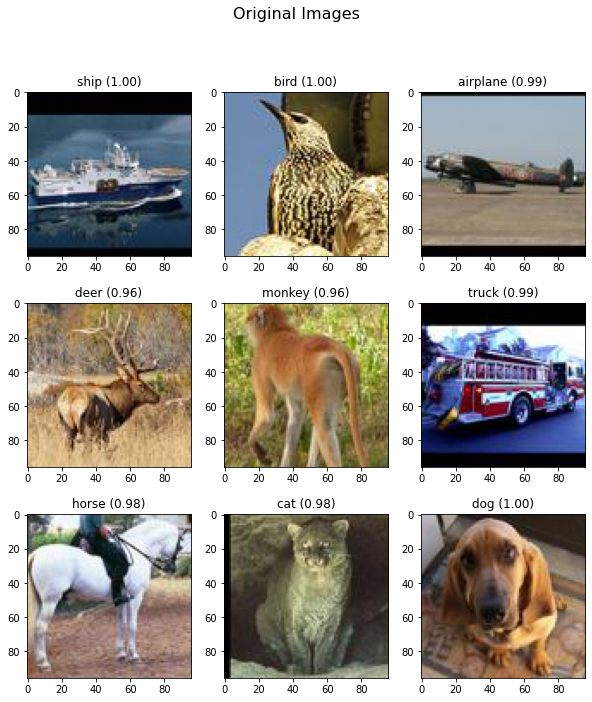
All good. We are ready to go!
Physical Attack Class
This class implements the functionality that is described in the introduction.
It mainly consists of a _setup_attack_graph method, which defines the noise variable and the required operations and a generate method, which initializes the noise vector and loops over the epochs. Look through each function for a better understanding. We have commented all the important parts.
class PhysicalAttack():
    """
    This class implements a physical attack.
    During the attack, the noise is optimized within a certain mask in a way that the attack is successful.
    To make the attack potentially printable, colors for the noise can be set.
    """
    def __init__(self, img_rows, img_cols, depth, n_classes, noisy_input_clip_min,
                noisy_input_clip_max, attack_lambda, print_lambda, lr, model, targeted):

        # input image data
        self.img_rows = img_rows
        self.img_cols = img_cols
        self.depth = depth

        # this class is optimized for stl10 dataset
        self.n_classes = n_classes

        # clip the noise between 0 and 1 (for images)
        self.noisy_input_clip_min = noisy_input_clip_min
        self.noisy_input_clip_max = noisy_input_clip_max

        # regularization loss for the noise. Currently not used (is 0)
        self.attack_lambda = attack_lambda

        # loss weight for the printable colors
        self.print_lambda = print_lambda

        # learning rate
        self.lr = lr

        # model we want to attack
        self.model = model

        # this holds the function we have to call after building the attack graph
        self.train = None

        # variable for the noise
        self.noise = None

        # boolean, true if we want a targeted attack
        self.targeted = targeted

        # set allowed params, which the user can modify
        self.attack_params = list(self.__dict__.keys())

        # build the attack graph
        self._setup_attack_graph()

    def set_params(self, **kwargs):
        """
        This method sets the allowed attributes
        """

        for key, value in kwargs.items():
            if key in self.attack_params:
                setattr(self, key, value)
                print(key, value)
            else:
                raise KeyError("Unkown property ", key)
        return True

    def _l1_norm(self, tensor):
        """
        This method calculates the l1 norm
        :param tensor masked noise
        """
        return tf.reduce_sum(tf.abs(tensor))

    def _setup_attack_graph(self):
        """
        This method builds the attack graph by defining the placeholders and operations
        """

        # PLACEHOLDERS
        image_in = k.placeholder(dtype=tf.float32, shape = (None, self.img_rows, self.img_cols, self.depth))
        attack_target = k.placeholder(dtype=tf.float32, shape = (None, self.n_classes))
        noise_mask = k.placeholder(dtype=tf.float32, shape=(self.img_rows, self.img_cols, self.depth))
        printable_colors = k.placeholder(dtype=tf.float32, shape=(None,self.img_rows, self.img_cols, self.depth))
        noisy_input_clip_min = k.placeholder(dtype=tf.float32, shape=None)
        noisy_input_clip_max = k.placeholder(dtype=tf.float32, shape=None)
        attack_lambda = k.placeholder(dtype=tf.float32, shape=None)
        print_lambda = k.placeholder(dtype=tf.float32, shape=None)

        # Noise variable --> This is getting optimized
        self.noise = k.variable(tf.random_uniform([self.img_rows, self.img_cols, self.depth], 0.0, 1.0),
                    name='noise')

        # multiply noise with mask
        noise_mul =tf.multiply(noise_mask, self.noise)

        # clip noise_mul for printing
        noise_mul_clip = tf.clip_by_value(noise_mul, noisy_input_clip_min, noisy_input_clip_max)

        # get the inverse mask, build the sum of masked noise + inverse masked image
        inverse_masks = 1.0 - noise_mask
        noise_inputs = tf.clip_by_value(tf.add(image_in*inverse_masks, noise_mul),
                                        noisy_input_clip_min, noisy_input_clip_max)

        # get the prediction of the white box for the current noise
        adv_pred = self.model(noise_inputs)

        ####
        # REGULARIZATION LOSS
        ####
        reg_loss = self._l1_norm(noise_mul)

        ####
        # CLASSIFICATION LOSS
        ####
        loss_function = k.categorical_crossentropy
        loss_f = loss_function(attack_target, adv_pred, from_logits=False)[0]
        # if targeted is false, than attack_target holds the g.t., therefore take loss inverse
        if not self.targeted:
            # adding small amount to avoid division by zero
            loss = 1/(loss_f+1e-3)
        else:
            loss = loss_f

        ####
        # PRINTABILITY LOSS
        # 1. calculate the differences between pixel values in mask and every allowed color
        # 2. build the sum for each pixel difference
        # 3. Build the product, because its enough if the noise is close to only one class
        # 4. Reduce to sum
        ####
        printab_pixel_element_diff= tf.squared_difference(noise_mul, printable_colors*noise_mask)
        printab_pixel_diff = tf.reduce_sum(printab_pixel_element_diff, 3)
        printab_reduce_prod = tf.reduce_prod(printab_pixel_diff, 0)
        printer_error = tf.reduce_sum(printab_reduce_prod)

        ####
        # ADV LOSS
        ####
        adv_loss = loss + attack_lambda * reg_loss + print_lambda*printer_error # + reg_loss

        # Adam opimizer to optimize the variable noise
        opt = tf.keras.optimizers.Adam(learning_rate=self.lr,epsilon=1e-08)
        updates = opt.get_updates(adv_loss, [self.noise])

        # define keras function. This is called from generate method
        self.train = k.function([image_in, attack_target, noise_mask, printable_colors,
                                noisy_input_clip_min, noisy_input_clip_max,
                                attack_lambda, print_lambda],
                                [adv_loss, noise_inputs, loss, reg_loss, printer_error, noise_mul_clip, loss_f], updates=updates)

    def generate(self, n_epochs, img, target, mask, print_colors, verbose=True):
        """
        This method starts the attack
        :param n_epochs     Define the number of epochs we want to optimize the noise
        :param img          Attack image
        :param target       Target list. If targeted is false, this holds the g.t.
        :param mask         images of the masks
        :param print_colors images containing the allowed colors

        :return noisy_input The final output of the attack. This is the attack image + noise
        """

        # first initialize the noise variable
        k.get_session().run(tf.variables_initializer([self.noise]))

        if verbose:
            # optimize noise over n_epochs
            for i in trange(n_epochs):

                # do one step
                loss_all, noisy_input, loss_cat, loss_reg, loss_print, clipped_noise, losses_f = self.train([img, target, mask, print_colors,
                                                                         self.noisy_input_clip_min, self.noisy_input_clip_max,
                                                                         self.attack_lambda, self.print_lambda])

                if i % 200 == 0:
                    print()
                    print(f"loss all {loss_all}, loss prediction: {loss_cat}, loss printer: {loss_print}")
                    plt.title("Current Noise")
                    plt.imshow(clipped_noise.reshape(96, 96, 3))
                    plt.show()
        else:
            # optimize noise over n_epochs
            for i in range(n_epochs):

                # do one step
                loss_all, noisy_input, loss_cat, loss_reg, loss_print, clipped_noise, losses_f = self.train([img, target, mask, print_colors,
                                                                         self.noisy_input_clip_min, self.noisy_input_clip_max,
                                                                         self.attack_lambda, self.print_lambda])

        return  noisy_input
Define GUI with Jupyter Widgets
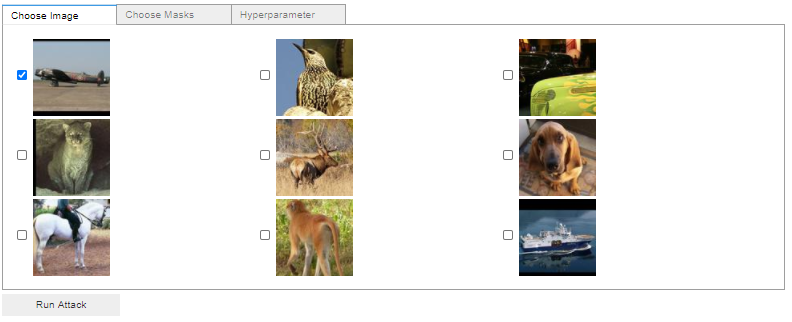
To make the configuration as easy as possible you are now going to build a small user interface with the Jupyter Widgets. The user interface should let the user:
- Select one of the nine input images
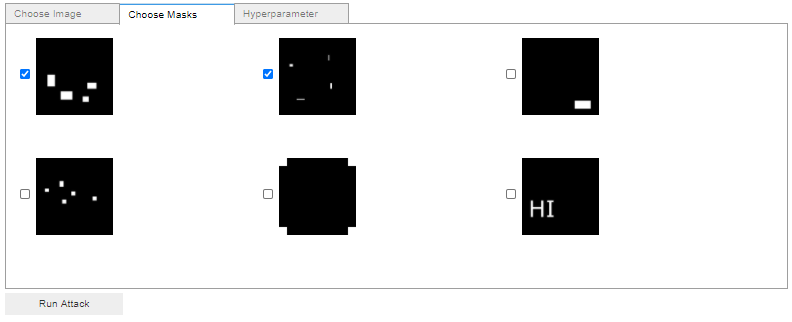
- Choose different masks
- Run targeted and untargeted attacks
- Select the target class in case of a targeted attack
- Set training parameters like learning rate, training epochs
- Enable and disable the inclusion of the printer error and set hyperparameters like printable colors or $\lambda_{printer}$
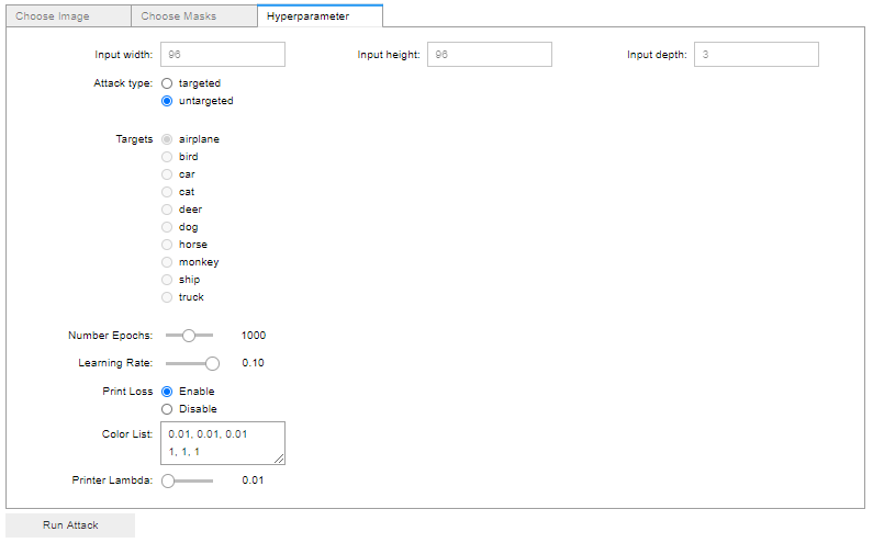
The final GUI should have three tabs. First, the user selects the input image, the masks and finally the hyperparameters. To give you a better idea of what our goal is, take a look at the following images:
Helper function
First, define a function row to create checkboxes with images as labels. Then we’re going to create some listeners (img_checkbox_listener, printer_loss_listener, attack_type_listener) on sliders and checkboxes to recognize events. The last two functions are used to read in the input images and the masks and to create image representations of the user-defined colors. Have a closer look at each method.
def row(descr):
    """
    This is used to create images and checkboxes next to each other
    """
    return widgets.Checkbox(description=descr, value=False, indent=False)


def img_checkbox_listener(change):
    """
    This method manually allows only one checkbox to be checked.
    :param change    dictionary with changes
    """
    curr_descr = change["owner"].description
    for rb in rbs_imgs:
        if rb.description != curr_descr:
            rb.value=False


def printer_loss_listener(change):
    """
    This listener enables or disbables the printer hyperparameters
    if we don't want to include printable colors
    :param change    dictionary with changes
    """
    if change["new"] == "Enable":
        colors.disabled=False
        print_lambda_slider.disabled = False
    elif  change["new"] == "Disable":
        colors.disabled=True
        print_lambda_slider.disabled = True


def attack_type_listener(change):
    """
    This listener enables or disbables the target selection
    :param change    dictionary with changes
    """
    if change["new"] == "untargeted":
        targets.disabled=True
    elif  change["new"] == "targeted":
        targets.disabled=False


def _read_img(descr_list, is_mask, w, h, d):
    """
    This method is used to read in attack images or masks
    :param descr_list    list of html descriptions of images
    :param is_mask       true, if image is a mask
    :param w             width of image
    :param h             height if image
    :param d             depth of image
    """

    # descriptions look like <img src='...'>. We extract the image path
    pattern = re.compile(r"'(.*?)'")

    # check if image is a mask
    if is_mask:
        masks = []
        # load all masks
        for m in descr_list:
            path = re.findall(pattern, m)[0]
            mask = cv2.imread(path)
            mask = mask/255.
            masks.append(mask)
        return masks
    else:
        # load attack image
        path = re.findall(pattern, descr_list[0])[0]
        img = plt.imread(path)
        img = img/255.
        img = img.reshape(1, w, h, d)
        return img, path


def _load_color_list(colors_str, w, h):
    """
    Load the printable colors and convert them into images with w, h, (d).
    For each color an image is generated that only contains pixel with that color
    :param colors_str       Textarea from the gui, containing the defined colors
    :param w                width of image
    :param h                height of image

    :return p               colored images
    """

    # container for colored images
    p = []

    # iterate over each color in the string
    for c in colors_str.split("\n"):
        p.append(c.split(","))

    # generate w, h, d images
    p = map(lambda x: [[x for _ in range(w)] for __ in range(h)], p)
    p = np.array(list(p)).astype(float)

    return p
Create GUI elements
First, build the row elements of the first tab, where the user can select the input image. Secondly, add a checkbox listener to automatically deselect an option if another one is clicked. After that, create the checkboxes for the mask selection on the second tab and finally create all the sliders and selection options for the hyperparameter selection tab.
####
# Create checkboxes for the input images
# We set 9 images fix from stl10 dataset
####
rbs_imgs = (row("<img src='physical_attack_data/imgs_gui/airplane.jpg'>"), row("<img src='physical_attack_data/imgs_gui/bird.jpg'>"),
            row("<img src='physical_attack_data/imgs_gui/car.jpg'>"), row("<img src='physical_attack_data/imgs_gui/cat.jpg'>"),
            row("<img src='physical_attack_data/imgs_gui/deer.jpg'>"), row("<img src='physical_attack_data/imgs_gui/dog.jpg'>"),
            row("<img src='physical_attack_data/imgs_gui/horse.jpg'>"), row("<img src='physical_attack_data/imgs_gui/monkey.jpg'>"),
            row("<img src='physical_attack_data/imgs_gui/ship.jpg'>"))
radio_buttons_imgs = widgets.HBox([*rbs_imgs], layout=Layout(height="300px", width='100%', display='inline-flex',flex_flow='row wrap'))
for rb in rbs_imgs:
    rb.observe(img_checkbox_listener)


# Create GUI elements
# Create checkboxes for the masks
####
rbs = ( row("<img src='physical_attack_data/masks/mask1.png'>"), row("<img src='physical_attack_data/masks/mask2.png'>"),
        row("<img src='physical_attack_data/masks/mask3.png'>"), row("<img src='physical_attack_data/masks/mask4.png'>"),
        row("<img src='physical_attack_data/masks/mask5.png'>"), row("<img src='physical_attack_data/masks/mask6.png'>"))
radio_buttons = widgets.HBox([*rbs], layout=Layout(height="300px", width='100%', display='inline-flex',flex_flow='row wrap'))


####
# Create widgets for hyperparametrs
####
# width of image (currently fixed to stl10)
w_input = widgets.Text(
    value='96',
    description='Input width:',
    style ={'description_width': '150px'},
    disabled=True
)
# height of image (currently fixed to stl10)
h_input = widgets.Text(
    value='96',
    description='Input height:',
    style ={'description_width': '150px'},
    disabled=True
)
# depth of image (currently fixed to stl10)
d_input = widgets.Text(
    value='3',
    description='Input depth:',
    style ={'description_width': '150px'},
    disabled=True
)
input_dims = HBox([w_input, h_input, d_input])

# number of classes in stl10
n_classes = widgets.Text(
    value='10',
    description='Number of classes:',
    style ={'description_width': '150px'},
    disabled=True
)

# number of epochs slider
n_epochs = widgets.IntSlider(
    value=1000,
    min=100, max=2000, step=100,
    description='Number Epochs:',
    style ={'description_width': '150px', 'width':'100%'}
)

# printer loss slider
print_lambda_slider = widgets.FloatSlider(
    value=0.01,
    min=0, max=1, step=0.01,
    description='Printer Lambda:',
    style ={'description_width': '150px', 'width':'100%'}
)

# learning rate slider
lr = widgets.FloatSlider(
    value=0.1,
    min=0.01, max=0.1, step=0.01,
    description='Learning Rate:',
    style ={'description_width': '150px'}
)

# printable colors textarea
colors = widgets.Textarea(
    value='0.01, 0.01, 0.01\n1, 1, 1',
    description='Color List:',
    style ={'description_width': '150px'}
)

# attack type radio button
attack_type = widgets.RadioButtons(
    options=['targeted', 'untargeted'],
    description='Attack type:',
    disabled=False,
    style ={'description_width': '150px'}
)
attack_type.observe(attack_type_listener)

# targets radio buttons
targets = widgets.RadioButtons(
    options=class_list,
    description="Targets",
    disabled=False,
    style ={'description_width': '150px'}
)

# print attack boolean radio button
printer_attack = widgets.RadioButtons(
    options=['Enable', 'Disable'],
    description='Print Loss',
    disabled=False,
    style ={'description_width': '150px'}
)
printer_attack.observe(printer_loss_listener)
‘Start Button’ Listener
The whole process is started as soon as the Run Attack-Button is pressed. Therefore, we’ve to listen on that event.
Inside this handler, check if the user has selected an input image and at least one mask. If not, the attack cannot be started.
If the selection is valid, the input image and the mask is read in. The true label of the input image is extracted from the filename. If the user wants to run a targeted attack, the selection from the radio buttons will be set as a target. If the user wants to run an untargeted attack, the extracted true label of the image will be taken into account. Before the attack can be executed, the user-defined colors have to be loaded. After these steps, you can create an instance of the PhysicalAttack class and start the attack.
def attack_button_listener(btn_object):
    """
    This method is the starting point of the attack. It gets triggered as soon as the user clicks on the attack button
    """
    print("Starting the attack...")

    # get attack image description
    selected_imgs = []
    for i, item in enumerate(rbs_imgs):
        if item.value:
            selected_imgs.append(item.description)

    # user needs to select one image
    if len(selected_imgs) == 0:
        print("Please select at least one image")
    else:
        # read in image
        img, path = _read_img(selected_imgs, False, int(w_input.value), int(h_input.value), int(d_input.value))

        # true label is encoded inside the file name
        path = path.split("/")[2]
        true_label = path.split(".")[0]

        # get masks descriptions
        selected_masks = []
        for i, item in enumerate(rbs):
            if item.value:
                selected_masks.append(item.description)

        # user needs to select at least one mask
        if len(selected_masks) == 0:
            print("Please select at least one mask")
        else:

            #read in mask
            masks = _read_img(selected_masks, True, int(w_input.value), int(h_input.value), int(d_input.value))

            # generate target vectors
            target = np.zeros((1, len(class_list)))

            # if targeted attack, then take the user defined target
            # else take the g.t. as target
            if attack_type.value == "targeted":
                target[0][class_list.index(targets.value)] = 1
            else:
                target[0][class_list.index(true_label)] = 1

            # this is our white box model
            model = load_model("../final_models/vgg16_stl10.h5")

            # load the printable colors
            p = _load_color_list(colors.value, int(w_input.value), int(h_input.value))

            # check if we want to include colors inside the attack
            print_lambda = 0
            if printer_attack.value == "Enable":
                print_lambda =  print_lambda_slider.value

            ####
            # Instatiate the PhysicalAttack class and set parameter
            # Attack lambda is set to zero, because we don't care about how much we see the noise
            ####
            attack = PhysicalAttack(img_rows=int(h_input.value),
                                    img_cols=int(w_input.value),
                                    depth=int(d_input.value),
                                    n_classes=int(n_classes.value),
                                    noisy_input_clip_min = 0,
                                    noisy_input_clip_max = 1,
                                    attack_lambda = 0,
                                    print_lambda = float(print_lambda),
                                    lr = float(lr.value),
                                    model=model,
                                    targeted = attack_type.value == "targeted")

            # container for generated images
            adv_images = []
            for i, m in enumerate(masks):
                print(f"Mask {i+1}", "#"*20)
                # do the attack of n_epochs for each mask
                adv_images.append(attack.generate(img=img,
                                            n_epochs=int(n_epochs.value),
                                            target=target,
                                            mask=m,
                                            print_colors=p,
                                            verbose=1))
            # plot all generated images
            plot_physical_adv(model, int(w_input.value), int(h_input.value), int(d_input.value),
                              adv_images, target, save=True, name=true_label, attack_type=attack_type.value)
‘Start Button’ GUI element
What remains to be done is to create a button and add the ‘Start Button’ listener.
# Create attack button and listen to it with the above function
button = widgets.Button(
    description='Run Attack',
)
button.on_click(attack_button_listener)
Run Attacks
As a starting point, we’re going to give you some examples of attacks and show you what you can derive from their results. Of course, you can also start directly with your own experiments.
Guided experiments
1. Airplane
- Choose the airplane as input image
- In the first row, choose the first and the last mask
- Set an untargeted attack with $600$ epochs, $lr=0.1$ and disable the inclusion of printer error
What can you learn from the output?
You should see that with the first mask we can create a perturbation, which fools our white-box model because it predicts the car as a truck. With the second mask we are not able to fool our model. It is still pretty sure that the image shows an airplane. This directly suggests that not every mask works equally well. That makes sense because different masks also cover different areas of the input image.
2. Deer
- Choose the deer as input image
- Choose the mask that shows the text ‘HI’
- Set a targeted attack with target class airplane
- Set $600$ epochs and $lr=0.1 $
- Add printable colors:$ 0.01, 0.01, 0.01 $ and $1, 1, 1 $ and set $\lambda_{printer}=0.3$
- After the first run, change $\lambda_{printer}$ to be $1.0$
What can you learn from the output?
First thing you should see is that we force our perturbation to be close to black and white pixels. In the first experiment we didn’t have such a constraint. With $\lambda_{printer}=0.3$ the attack is successful. The deer gets classified as airplane. If we increase $\lambda_{printer}$ to $1.0$ , we cannot achieve this anymore. We put so much weight on the minimization of the printer error that the model can no longer learn a perturbation to fool the model. This shows you that you have to find the right weighting of the two losses. It can also be concluded that the more latitude, i.e. colors of the pixels, the algorithm has available to generate perturbation, the higher the chance of success. Finally, you can also see that there aren’t restrictions in the form of the masks. Masks can have rectangular shapes, but also be letters or any other symbols.
3. Monkey
- Choose the monkey as input image
- Choose the first mask in the second row
- Set an untargeted attack
- Set $600$ epochs and $lr=0.1 $
- Add only one printable color:$ 1, 1, 1 $ and set $\lambda_{printer}=1.0$
What can you learn from the output?
In this case, we can create a perturbation that has pixel values very close to white pixels and still fool the classification model. With (nearly) only one color we are able to create a successful attack. Of course, this won’t work for all images, but this shows that you should examine each image separately because there are different settings per image which work well and badly.
Now try your own attacks
Your resulting images are saved in ./generated_advs.
# build gui
tab_rb_imgs = VBox(children=[radio_buttons_imgs])
tab_rb = VBox(children=[radio_buttons])
tab_hp = VBox(children=[input_dims,

                      attack_type,
                        targets,
                        n_epochs,
                        lr,
                        printer_attack,
                        colors,
                       print_lambda_slider

                       ])

gui = widgets.Tab(children=[ tab_rb_imgs, tab_rb, tab_hp])
gui.set_title(0, 'Choose Image')
gui.set_title(1, 'Choose Masks')
gui.set_title(2, 'Hyperparameter')
VBox(children=[gui, button])
Validate Different Masks on 2000 Test Images
As the first guided experiment already shows, there are certainly differences in the success rates of the individual masks. Therefore, we have picked three different masks to test them on 2000 test images. You may also choose other masks.
Mask 1

Mask1 consists of large areas. Moreover, it is positioned around the center of the images. Therefore, there is a high possibility that the mask will cover some parts of the object of interest.
Mask 2

Mask2 is also located in the center, but is clearly smaller than mask1.
Mask 3

Mask3 covers larger area, but is located at the corner.
Expectations
Which mask do you think will work best?
We expect the mask1 to perform best because we believe that the chances of success will be better if we cover parts of the object. Mask2 might be better than mask3 because of its position, but there only few pixel we can add noise to.
Load the STL10 dataset
Let’s start by loading the dataset.
# define stl10 class list and preprocess dataset
class_list = ["airplane", "bird", "car", "cat", "deer", "dog", "horse", "monkey", "ship", "truck"]
num_classes = 10

# define width, height and dimension of images
w, h, d = 96, 96, 3

# The data, split between train and test sets:
(x_test, y_test), (x_train, y_train)= stl10.load_data()
print('x_train shape:', x_train.shape)
print(x_train.shape[0], 'train samples')
print(x_test.shape[0], 'test samples')

# Convert class vectors to binary class matrices.
# Stl10 datasets starts with class 1, not 0
y_train = keras.utils.to_categorical(y_train-1, num_classes)
y_test = keras.utils.to_categorical(y_test-1, num_classes)

# Scale data between 0 and 1
x_train = x_train.astype('float32')
x_test = x_test.astype('float32')
x_train /= 255
x_test /= 255
x_train shape: (8000, 96, 96, 3)
8000 train samples
5000 test samples
Run attack for 2000 images
To ensure the easiest case of the attacks, disable the inclusion of the printer error and use an untargeted attack. Run each attack for 400 epochs.
The process of creating three adversarial images for every single image in our test scope takes some time (several hours, depending on your machine). Therefore, we dumped our results in a pickle file and load the adversarial images from the disk. To speed up the process you can reduce the number of images to be included in the attack. To do so, just change the number_of_images variable.
# number of images included in the validation
number_of_images = 2000

# Instatiate attack class and read in masks
# define the class
attack = PhysicalAttack(img_rows=96,
                        img_cols=96,
                        depth=3,
                        n_classes=10,
                        noisy_input_clip_min = 0,
                        noisy_input_clip_max = 1,
                        attack_lambda = 0,
                        print_lambda = 0,
                        lr = 0.1,
                        model=model,
                        targeted = False)
# load the masks
masks = []
mask_paths = ["./physical_attack_data/masks/mask1.png", "./physical_attack_data/masks/mask2.png", "./physical_attack_data/masks/mask3.png"
for m_path in mask_paths:
    mask = cv2.imread(m_path)
    mask = mask/255.
    masks.append(mask)
Save the pickle file in physical_attack_data/pickle_dumps/adv_on_<number_of_images>.p in order to load it afterwards.
# Attack the Images, this takes long for 2000 images!
if not os.path.isfile(f"physical_attack_data/pickle_dumps/adv_on_{number_of_images}.p"):
    # storage for all adv images
    all_advs = []
    # dummy colors
    p = _load_color_list("1, 1, 1", int(w_input.value), int(h_input.value))
    for i in trange(len(x_test[:number_of_images])):
        t_image = x_test[i]
        adv_images = []
        for j, m in enumerate(masks):
            # do the attack of n_epochs for each mask
            adv_images.append(attack.generate(img=t_image.reshape(1, 96, 96, 3),
                                        n_epochs=400,
                                        target=y_test[i:i+1],
                                        mask=m,
                                        print_colors=p,
                                        verbose=0))
        all_advs.append(adv_images)

    # dump the results
    all_advs = np.array(all_advs)
    pickle.dump( all_advs, open( f"physical_attack_data/pickle_dumps/adv_on_{number_of_images}.p", "wb" ))
    print(f"Dump new adversarial images")
else:
    all_advs = pickle.load(open( f"physical_attack_data/pickle_dumps/adv_on_{number_of_images}.p", "rb" ))
    print("Load existing dump of adversarial images")
Load existing dump of adversarial images
Baseline
On the first 2000 images, our white-box model has an accuracy of ~79%.
print(f"Baseline of first {number_of_images} images: ", model.evaluate(x_test[:number_of_images], y_test[:number_of_images])[1])
2000/2000 [==============================] - 2s 769us/step
Baseline of first 2000 images:  0.7854999899864197
Success rate of the masks
For each mask, the model predicts the class label. After that, subtract the accuracy of the model from 1 to get the success rate.
print(all_advs.shape)

# first extract images per mask and do reshape
all_advs = np.array(all_advs)
first_masks = all_advs[:, 0].reshape(-1, 96, 96, 3)
second_masks = all_advs[:, 1].reshape(-1, 96, 96, 3)
third_masks = all_advs[:, 2].reshape(-1, 96, 96, 3)

# check model acc, success rate is 1-model acc
print("Succes rate of mask 1: ", 1- model.evaluate(first_masks, y_test[:number_of_images])[1])
print("Succes rate of mask 2: ", 1- model.evaluate(second_masks, y_test[:number_of_images])[1])
print("Succes rate of mask 3: ", 1- model.evaluate(third_masks, y_test[:number_of_images])[1])
(2000, 3, 1, 96, 96, 3)
2000/2000 [==============================] - 1s 553us/step
Succes rate of mask 1:  0.9470000006258488

2000/2000 [==============================] - 1s 555us/step
Succes rate of mask 2:  0.5785000026226044

2000/2000 [==============================] - 1s 554us/step
Succes rate of mask 3:  0.5985000133514404
| Mask | Attack Type | Printer Loss | Success rate (%) | #Images |
|---|---|---|---|---|
| Mask1 | untargeted | disabled | 94.7 | 2000 |
| Mask2 | untargeted | disabled | 57.8 | 2000 |
| Mask3 | untargeted | disabled | 59.8 | 2000 |
Observations:
As expected, the first mask has the highest success rate. 94.7% of the 2000 test images are wrongly classified. This increases the suspicion that centered masks are more successful. But the noise area must also be large enough. Mask2 is also centered, but has a much lower success rate compared to Mask1. Mask3 shows that only a large area is not always enough to fool the classification model. The combination of both metrics (position and size) leads to success. If you want to be correct, you would have to subtract the pictures where the model was already wrong before the attack from the success rate. But in this experiment, it was only about comparing the performances of the masks.
Plot some examples
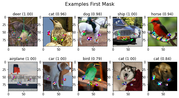
Here you can plot 10 images per mask. Make sure that you adjust the indices in case you’ve modified number_of_images.
You can see that the images of the first mask always lead to wrong predictions.
plot_images(first_masks[20:30], 5, 2, title="Examples First Mask", model=model, size=(10, 5))
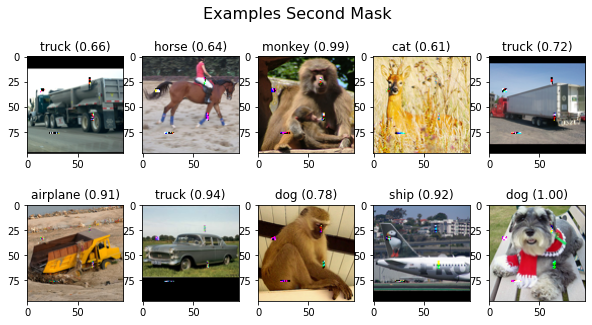
plot_images(second_masks[700:710], 5, 2, title="Examples Second Mask", model=model, size=(10, 5))
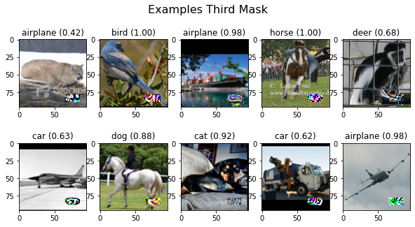
plot_images(third_masks[1800:1810], 5, 2, title="Examples Third Mask", model=model, size=(10, 5))
Let us Put the Attack on a Physical Level
So far, you have created a perturbation for a certain area of the image. But does it work in the real world? What about the assumption that the effectiveness of the noise is lost by printing it out?
We don’t have a perfect example here because you can’t really put a sticker on a deer. But the idea is transferable to e.g. traffic signs. In order to test the physical usability without much effort, you can do the following:
- Calculate a perturbation with our implementation
- Print both, the original image and the generated noise, separately
- Cut out the areas of perturbation and place them on the original image. Take care to keep the positions as good as possible
- Take a picture with a mobile phone, scale the picture back to 96x96 and let the model make a prediction on it. Through the process of taking picture with the mobile phone, we get different light conditions, viewing angles and another quality in general compared to the original image in the dataset
First example: Targeted attack on deer
The first row shows the digital representations, the second row the printed ones.
# load digital and printed images
# original digital image
img_org = plt.imread("./physical_attack_data/imgs_adv/deer.jpg")
img_org = img_org/255.

# original attack image
attack_org = plt.imread("./physical_attack_data/imgs_adv/deer_airplane.jpg")
attack_org = attack_org/255.

# photo original image
img_photo = plt.imread("./physical_attack_data/imgs_adv/deer_org.jpg")
img_photo = img_photo/255.


# photo attack image
attack_photo = plt.imread("./physical_attack_data/imgs_adv/deer_adv.jpg")
attack_photo = attack_photo/255.


plot_images(np.array([img_org, attack_org, img_photo, attack_photo]), columns=2, rows=2, model=model, title="Deer Example (Success)", size=(15, 8))
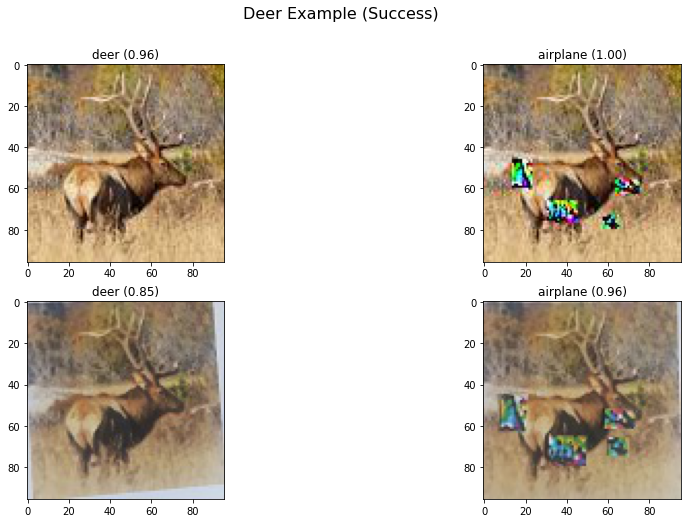
Observations: Although the noise can include any colors, the attack still works with the printed and photographed image. Cool, isn’t?
Second example: Untargeted attack on airplane
The first row shows the digital representations, the second row the printed ones
# load digital and printed images
# original digital image
img_org = plt.imread("./physical_attack_data/imgs_adv/airplane.jpg")
img_org = img_org/255.

# original attack image
attack_org = plt.imread("./physical_attack_data/imgs_adv/airplane_ship.jpg")
attack_org = attack_org/255.

# photo original image
img_photo = plt.imread("./physical_attack_data/imgs_adv/airplane_org.jpg")
img_photo = img_photo/255.


# photo attack image
attack_photo = plt.imread("./physical_attack_data/imgs_adv/airplane_adv_ship.jpg")
attack_photo = attack_photo/255.


plot_images(np.array([img_org, attack_org, img_photo, attack_photo]), columns=2, rows=2, model=model, title="Airplane untargeted (Success)", size=(15, 8))
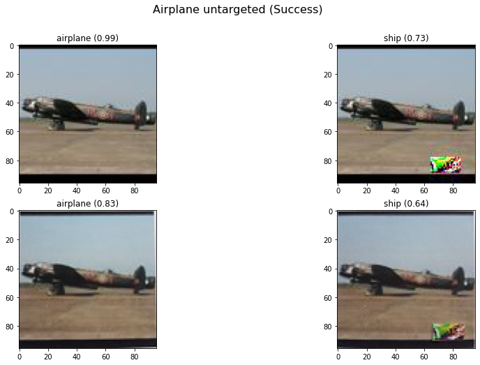
Observations: Again, the attack still works. The airplane is classified as ship. But there is a slight decrease in the confidence.
Third example: Targeted attack on airplane
The first row shows the digital representations, the second row the printed ones
# load digital and printed images
# original digital image
img_org = plt.imread("./physical_attack_data/imgs_adv/airplane.jpg")
img_org = img_org/255.

# original attack image
attack_org = plt.imread("./physical_attack_data/imgs_adv/airplane_horse.jpg")
attack_org = attack_org/255.

# photo original image
img_photo = plt.imread("./physical_attack_data/imgs_adv/airplane_org.jpg")
img_photo = img_photo/255.


# photo attack image
attack_photo = plt.imread("./physical_attack_data/imgs_adv/airplane_adv_horse.jpg")
attack_photo = attack_photo/255.


plot_images(np.array([img_org, attack_org, img_photo, attack_photo]), columns=2, rows=2, model=model, title="Airplane targeted (Failure)", size=(15, 8))
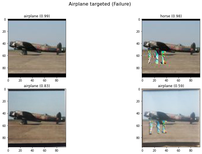
Observations: Although the generated mask leads to a very strong, false prediction in the digital world, the photographed image with the printed mask is not able to fool the classification model. At least, there is a decrease of ~40 percent in the confidence of the model prediction. There are several reasons why this attack does not work compared to the others. For one thing, it is more difficult to cut and position the mask correctly. In addition, the lighting conditions are slightly different.
Conclusion
In this tutorial you should have learned how to generate a perturbation in selected areas of an input image and also how to control the color of the noise. Let’s sum it up:
On physical attacks
- Basically, masks that cover larger area around the center of an image work best. At least for the images in the STL10, because the objects of interest are often located in the center.
- Disabling the inclusion of the printer error increases the chance that the attack will be successful in the digital world. Too large restriction on the color space leads to a strong minimization of the printer error, but not necessarily to a sufficient minimization of the crossentropy loss. You need to find a good balance and adapt the algorithm to your needs.
- The few printed attack images show that the effectiveness of the noise is not necessarily lost after printing it. But more tests are required for a scientific statement.
- Our printed attack images are not totally robust against light conditions and different viewing angles. To make them more robust you can use the pre-processing steps described in the introduction.
- There are some recent papers, such as the one entitled ImageNet-trained CNNs are biased towards texture, which discusses the fact that Deep Neuronal Networks don’t pay much attention to the outline of objects as expected, but to texture. This might be applied to our experiment, since we hardly change the shape of objects by using masks, but often a part of the mask lies within the objects and thus changes a part of the texture.
- It’s not quite easy to place the printed perturbation at the correct position. A small deviation might be enough to destroy the attack.
Where to look next
For us, this notebook has shown that robust attacks are not always that simple at the physical level. For one thing, it is clear that monochrome noise rarely leads to success. So you have to allow more diversity, but this makes the noise more noticeable. Additionally, one would have to test different positions of the masks. A further idea would be an algorithm that learns an optimal mask and its position and color by itself. For that, the work in One Pixel Attack for Fooling Deep Neural Networks [7], where researchers performed a one-pixel attack on images by finding the most influential pixel, could be extended to create masks automatically. Moreover, such masks let you identify influential areas in the input image. Not surprisingly, there is an overlap between the topics of adversarial attacks and visualization of learned features (that might lead to a better understanding of Neuronal Networks), because the masks could represent a certain feature that the model has learned, or at least cover the parts that are influential for a prediction.
Look at the next chapter, which is on Black-Box attacks!
Sources
[1] Robust Physical-World Attacks on Machine Learning Models
[2] Accessorize to a Crime: Real and Stealthy Attacks on
State-of-the-Art Face Recognition
[3] Adam: A method for stochastic optimization
[4] Deep Learning, S.82.86
[5] GTRSB
[6] ImageNet-trained CNNs are biased towards texture
[7] One Pixel Attack for Fooling
Deep Neural Networks