

Selected Topics #1: Adversarial Attacks
Chapter 3: Black-Box Attacks
This chapter implements the attack described in the paper “Practical Black-Box Attacks against Machine Learning”.[1]
Contents
- Introduction to Black-Box Attacks
- Prerequisites
- A Demonstration of Attack Transferability
- The Black-Box Attack
- Conclusion
- Sources
Introduction
We have now covered the white-box attacks “FGSM” and “PGD” in detail. These attacks are very effective on their own - but they have one significant weakness: To use them, the attacker must know everything about the target model. Specifically, they need:
- the target architecture,
- the target parameters,
- the dataset on which the target was trained.
In other words, an attacker needs a full local copy of the target model, training data and all. At first glance this seems like great news for defenders: You can hide the model from attackers, so they can’t craft adversarial samples. This concept is called gradient masking. Problem solved, attack averted, case closed?
Well, unfortunately no. There is another class of adversarial attack methods: Black-box attacks. These methods are built on the assumption, that an attacker doesn’t know much about the target at all. There are many different black-box methods and approach vectors out there, but let’s pick one [1] and find out how it works!
Substitute Model Attack
Let $O$ be some target classifier that is hidden behind an API. $O$ is called an oracle. We don’t know much about $O$ - only that it takes some input $x$ and returns some class prediction $y$ . $O$ cannot be blindly attacked with FGSM or PGD.
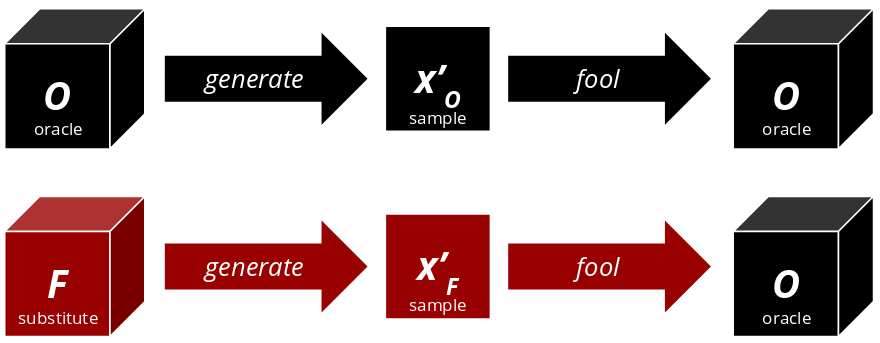
Transferability
The key concept to make this attack work is called transferability: So long as two classifiers share the same domain (e.g. image classification), the same adversarial noise $\delta$ may be effective on both of them. They don’t need to be exact copies of each other. Suppose one can somehow create a substitute model $F$ that is similar to $O$ . One could now use $F$ to craft an adversarial sample $x'_F$ that is effective on $O$ ! The methods FGSM and PGD we’ve covered earlier happen to have this transferability property.
Assumptions
No attack can work completely without knowledge about the target. The classifier may be hidden but an attacker can still make some informed assumptions about architecture and dataset. Such assumptions include:
- Model domain (image, text, sound etc.)
- Network architecture and complexity (Simple CNN, VGG, Inception, ResNet etc.)
- What dataset was likely used for training (MNIST, Cifar10/100, STL10 etc.)
- How much/fast the oracle can be queried without drawing attention.
According to the paper authors, these assumptions don’t need to be spot-on. As long as they are close enough, the adversarial samples generated to fool our homebrew classifier $F$ should also apply to the black-box classifier $O$ .
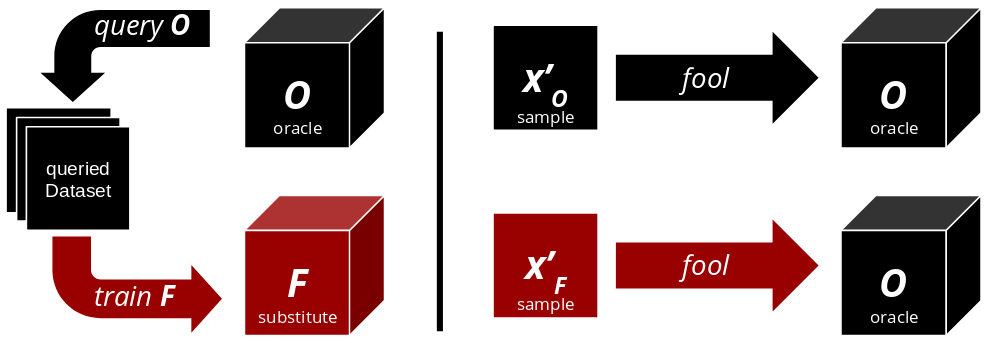
The Basic Algorithm
This is the short version of the algorithm that you will implement. Points 1 and 2 require high level domain knowledge, to make reasonable assumptions. Once $F$ is successfully trained, one can use FGSM or PGD to craft adversarial examples $x'_F$ with it.
- Collect input data representative for the oracle’s domain.
- Select a substitute architecture.
- Query the oracle with the collected input data.
- Train the substitute classifier $F$ .
Prerequisites
Import Modules
Below are all of the modules that must be imported to run this tutorial. You will reuse the FGSM and PGD implementations from the first chapter, so be sure to copy them over! You will again use the Keras library for training. Apart from Keras you also need some TensorFlow-specific functions, for example to calculate the jacobian matrices on your model later.
# Code: Imports
import logging
import os

import keras.backend as k
import matplotlib.gridspec as gridspec
import matplotlib.pyplot as plt
import numpy as np
import requests
import seaborn as sns
import tensorflow as tf

from gradientAttack import FastGradientMethod, GradientAttack, ProjectedGradientDescent
from io import BytesIO
from IPython.display import clear_output
from keras import optimizers
from keras.datasets import mnist
from keras.layers import Activation, Conv2D, Dense, Flatten, MaxPooling2D
from keras.models import load_model, Model, Sequential
from keras.utils import to_categorical
from PIL import Image
from sklearn.metrics import confusion_matrix
from tensorflow.python.ops.parallel_for.gradients import batch_jacobian
from tqdm.keras import TqdmCallback
from tqdm.notebook import tqdm

# Suppress tensorflow warnings
os.environ['TF_CPP_MIN_LOG_LEVEL'] = '3'  # FATAL
logging.getLogger('tensorflow').setLevel(logging.FATAL)
Using TensorFlow backend.
Download the Data
First, you need yourself some data. For this tutorial, MNIST is appropriate because
- MNIST “oracle” APIs are easy to find,
- training models on MNIST is very fast,
- the referenced paper also uses it.[1] :)
MNIST images show written digits from 0 to 9. They have a resolution of 28x28 pixels and only one color channel.
# Code: Load data

# Define globals
num_classes = 10
class_list = range(num_classes)

# Load MNIST dataset:
(x_train, y_train), (x_test, y_test) = mnist.load_data()
print(f"Successfully loaded MNIST dataset with {x_train.shape[0]} training samples and {x_test.shape[0]} test samples.")
Successfully loaded MNIST dataset with 60000 training samples and 10000 test samples.
Access & Test the Oracle API
The oracle we’ve used is a ready-made pytorch model running on a torchserve API server. We used this great tutorial [2] to deploy it.
Using the function query oracle() one can send an image to the oracle. It then returns the prediction as a single integer.
You can choose the same oracle, deploy your own or even rent an oracle API from your cloud provider of choice. You’ll only need to change query_oracle() to work with your API.
Note: If the oracle is running locally, you could technically look inside it. Of course, doing so would defeat the purpose of this tutorial. In a real scenario, you wouldn’t control the API and couldn’t look inside anyway.
# Code: Functions to query the oracle
def query_oracle(sample):
    """
    Send a single classification query to the oracle.
    :param sample: sample image as numpy array (int) with shape (w, h) in [0, 255]
    :return:       predicted class as integer
    """
    buffer = BytesIO()
    image = Image.fromarray(sample)
    image.save(buffer, format='PNG')
    image_bin = buffer.getvalue()
    response = requests.post('http://127.0.0.1:8085/predictions/mnist', data=image_bin)
    return int(response.content.decode())

def get_oracle_predictions(X):
    """
    Call oracle function on an array of images.
    :param X: images as numpy array (int) with shape (-1, w, h) in [0, 255]
    :return:  predicted class as numpy array (int) with shape (-1)
    """
    preds = []
    for i in tqdm(range(X.shape[0])):
        preds.append(query_oracle(X[i]))
    return(np.array(preds))
Try it out
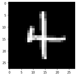
The following cell sends a random image from the MNIST test set to the oracle.
# Code: Sample prediction
sample = x_test[np.random.randint(x_test.shape[0])]
print(f"Oracle prediction: {query_oracle(sample)}")
plt.imshow(sample, cmap='gray');
Oracle prediction: 4
Confusion Matrix
Let’s evaluate the oracle’s performance, using the MNIST test set. This is to find out whether the black-box is actually any good at its task. To this end, we have it predict every image on the entire MNIST test set.
Technically an attacker doesn’t know that the model was trained on MNIST, but this is fine for demonstration purposes.
# Code: Oracle performance evaluation
def get_accuracy(y,y_hat):
    """
    Calculate the accuracy of a prediction array w.r.t some ground truth labels.
    :param y:     ground truth label as numpy array (int)
    :param y_hat: predicted label as numpy array (int)
    :return:      the accuracy of the prediction as float
    :note:        We cannot use evaluate() for the oracle, so this will do.
    """
    correct = np.where((y==y_hat),1,0)
    return correct.sum() / y.shape[0]

def plot_confusion_matrix(y, y_hat, title="Confusion matrix"):
    """
    Plot the confusion matrix of a prediction array w.r.t some ground truth labels.
    :param y:     ground truth label as numpy array (int)
    :param y_hat: predicted label as numpy array (int)
    """
    conf_mat = confusion_matrix(y, y_hat)
    # Normalize per ground truth label, display as percentage
    conf_mat_norm = conf_mat / conf_mat.astype(np.float).sum(axis=1, keepdims=True) * 100

    fig = plt.figure(figsize=(16, 6))
    gs = gridspec.GridSpec(1, 2)
    plt.tight_layout()
    fig.suptitle(title, fontsize = 16)

    ax0 = plt.subplot(gs[0,0])
    ax0.set_title(f'Counting {y_hat.shape[0]} samples')
    sns.heatmap(conf_mat, annot=True, fmt="d",cmap="Blues", ax=ax0, annot_kws={"fontsize":8})
    ax0.set_ylabel('True label')
    ax0.set_xlabel('Predicted label')

    ax1 = plt.subplot(gs[0,1])
    ax1.set_title('Prediction percentage per true class')
    sns.heatmap(conf_mat_norm, annot=True, fmt=".3g", cmap="Blues", ax=ax1, annot_kws={"fontsize":8})
    ax1.set_ylabel('True label')
    ax1.set_xlabel('Predicted label')
    return
# Code: Evaluate the oracle on MNIST (test) and plot its confusion matrix.
print(f"Querying the oracle on {x_test.shape[0]} images.")
y_hat_test = get_oracle_predictions(x_test)
print(f"Oracle accuracy on MNIST test set: {get_accuracy(y_test, y_hat_test)}")
plot_confusion_matrix(y_test, y_hat_test);
Querying the oracle on 10000 images.

Oracle accuracy on MNIST test set: 0.9912
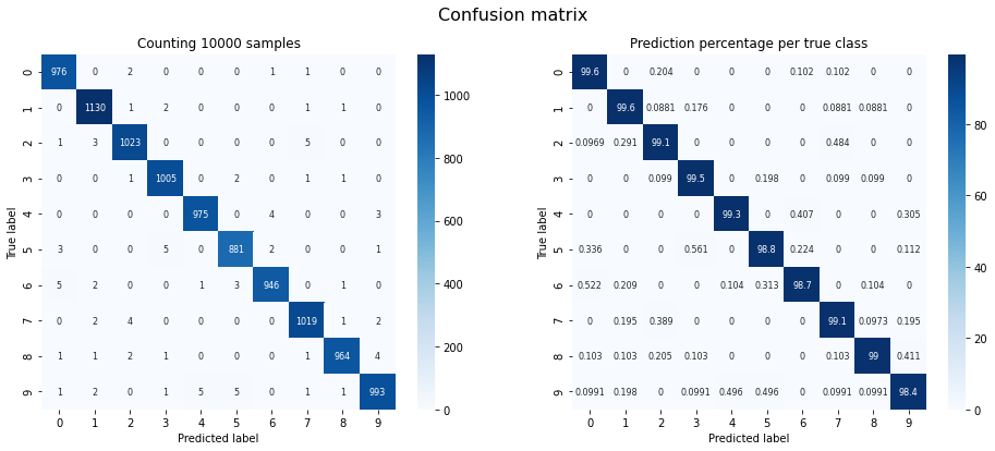
The confusion matrix shows the correlation between true class labels and predicted class labels (i.e. whether a ‘0’ was classified as a ‘0’, a ‘1’ as a ‘1’ and so on). The matrix on the left counts images, the one on the right shows percentages. Because most MNIST test samples were classified correctly, the matrices should show a diagonal line. Our chosen oracle has an accuracy of ~99.12%.
That will change soon.
Preprocessing
Finally, you must do some preprocessing. Input images are loaded as numpy arrays of integers with shape $(-1,28,28)$ in the interval $[0,255]$ . The oracle API accepts .PNG images with brightness values between 0 and 255, so that’s fine.
Keras models require more preprocessing: They should receive numpy arrays of shape $(-1,28,28,1)$
to account for the number of color channels. The arrays should also be normalized to the interval $[0,1]$
. Finally, the ground truth labels are one-hot encoded for compatibility with Keras’ Model.evaluate() method.
# Code: Preprocessing
w, h, d = 28, 28, 1 # Width, height and number of color channels

def preprocess(X, y):
    """
    Reshape, scale and encode data to feed to tensorflow graph.
    :param X: images as array with shape (-1,w,h) in [0, 255]
    :param y: labels as array with shape (-1)
    :return: X with shape (-1,w,h,d) in [0, 1], y onehot-encoded with shape (-1,10)
    """
    # Convert class vectors to binary class matrices.
    y_ohe = to_categorical(y, num_classes)
    # Scale data between 0 and 1
    X_scaled = X.astype('float32') / 255.
    # Add another dimension, since conv layers expect multiple input channels.
    X_scaled = np.reshape(X_scaled, (-1,w,h,d))
    return X_scaled, y_ohe

def back_to_image(X):
    """
    Reshape and scale images back for API compatibility.
    :param X: images as numpy array with shape (-1,w,h,d) in [0, 1]
    :return:  X with shape (-1,w,h) in [0, 255]
    """
    return (X[...,0]*255).astype(np.uint8)
Substitute Model: Transferability Demonstration
This first attack isn’t a true black-box attack yet, but only a demonstration of transferability. Once you’ve proven that transferability works, you will then turn it into a true black-box attack.
Attacker’s Knowledge
Let’s recall the knowledge on which to build your attack:
- Unknown
- oracle architecture
- oracle parameters
- Known
- domain: 28x28 grayscale images of digits
- training dataset: MNIST digits
In a true black-box scenario, the attacker doesn’t know that the oracle was trained on MNIST data. However, given its popularity, we are for now assuming that MNIST was used for training. The full algorithm requires us to actually query the oracle - you won’t do that yet. No worries, you will turn it into a true black-box attack later when we drop that assumption.
This first attack will be somewhat simpler than the true black-box attack planned for later. You only have to:
- choose an architecture.
- train the architecture.
Note: Technically you must send your training set to the oracle for labeling. However, MNIST is already labeled, so you might as well use those labels and save the time. This decision is somewhat naive, though: It assumes that the oracle would return those same labels, i.e. have a 100 percent accuracy.
We’ll say this assumption is close enough to the truth and run with it for this initial attack.
Step 1: Choose an Architecture for the Substitute Model
Given that the oracle operates on image data, it is a fair assumption that a convolutional architecture should be successful. The following model architecture has been taken directly from the paper. The batch size was the only hyperparameter not given, so we’re using the Keras default, 32.
# Code: Create substitute model graph
def build_model_A():
    """
    Create model A as substitute model architecture (Papernot et al. 2017).
    Paper link: https://arxiv.org/pdf/1602.02697.pdf
    :return: a tensorflow.keras.Model() object
    """
    batch_size = 32
    num_classes = 10

    model = Sequential()
    model.add(Conv2D(32, (2, 2), padding='same', input_shape=(28,28,1)))
    model.add(MaxPooling2D(pool_size=(2, 2)))
    model.add(Conv2D(64, (2, 2)))
    model.add(MaxPooling2D(pool_size=(2, 2)))
    model.add(Flatten())
    model.add(Dense(200))
    model.add(Activation('relu'))
    model.add(Dense(200))
    model.add(Activation('relu'))
    model.add(Dense(num_classes))
    model.add(Activation('softmax', name='y'))

    model.compile(
        loss='categorical_crossentropy',
        optimizer=optimizers.SGD(lr=0.01, momentum=0.9),
        metrics=['accuracy'])

    return model

model = build_model_A()
print(model.summary())
Model: "sequential_1"
_________________________________________________________________
Layer (type)                 Output Shape              Param #
=================================================================
conv2d_1 (Conv2D)            (None, 28, 28, 32)        160
_________________________________________________________________
max_pooling2d_1 (MaxPooling2 (None, 14, 14, 32)        0
_________________________________________________________________
conv2d_2 (Conv2D)            (None, 13, 13, 64)        8256
_________________________________________________________________
max_pooling2d_2 (MaxPooling2 (None, 6, 6, 64)          0
_________________________________________________________________
flatten_1 (Flatten)          (None, 2304)              0
_________________________________________________________________
dense_1 (Dense)              (None, 200)               461000
_________________________________________________________________
activation_1 (Activation)    (None, 200)               0
_________________________________________________________________
dense_2 (Dense)              (None, 200)               40200
_________________________________________________________________
activation_2 (Activation)    (None, 200)               0
_________________________________________________________________
dense_3 (Dense)              (None, 10)                2010
_________________________________________________________________
y (Activation)               (None, 10)                0
=================================================================
Total params: 511,626
Trainable params: 511,626
Non-trainable params: 0
_________________________________________________________________
None
Step 2: Train Substitute Model
See the code below for the training routine. Training for 10 epochs is more than enough to make the substitute model converge. Finally, evaluate the substitute model to see if it performs well enough.
# Code: Training function
def train_model(model, x_train, y_train, x_test, y_test, batch_size):
    """
    Train keras model
    :param model:   a tensorflow.keras.Model() object
    :param x_train: training inputs as array with shape (-1,w,h) in [0, 255]
    :param y_train: training labels as array with shape (-1)
    :param x_test:  test inputs as array with shape (-1,w,h) in [0, 255]
    :param y_test:  test labels as array with shape (-1)
    :return: training history
    """
    num_epochs = 10
    x_train, y_train = preprocess(x_train, y_train)
    x_test, y_test = preprocess(x_test, y_test)
    tqdm_callback = TqdmCallback(verbose=1)
    history = model.fit(
        x_train, y_train,
        batch_size = batch_size,
        epochs = num_epochs,
        validation_data = (x_test, y_test),
        shuffle = True,
        callbacks = [tqdm_callback],
        verbose = 0
    )
    return history
# Code: Train substitute model on MNIST
history = train_model(model, x_train, y_train, x_test, y_test, 32)
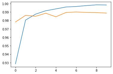
print("Accuracy and validation accuracy progress")
plt.plot(history.history["accuracy"])
plt.plot(history.history["val_accuracy"]);
Accuracy and validation accuracy progress
The two cells below are optional, in case you’d like to save the trained model to file.
# Code: Save model to file
save_dir = os.path.join(os.getcwd(), 'saved_models')
model_name = 'model_A_transferability'
if not os.path.isdir(save_dir):
    os.makedirs(save_dir)
model_path = os.path.join(save_dir, model_name)
model.save(model_path)
# Code: Load substitute model from file
#model = load_model("saved_models/model_A_transferability")
model = load_model("final_models/model_A_transferability")
Evaluate the performance of the substitute model.
def evaluate(model, X, y):
    """
    Evaluate the accuracy of a keras model.
    :param model: a tensorflow.keras.Model() object
    :param X:     images as numpy array with shape (-1,w,h) in [0, 255]
    :param y:     true class labels as numpy array with shape (-1)
    :return:      the accuracy of the prediction as float
    """
    X, y = preprocess(X, y)
    return model.evaluate(X, y, verbose=1)[1]

# Code: Evaluate the performance of the substitute model.
print(f"MNIST train accuracy: {evaluate(model, x_train, y_train):.4f}")
print(f"MNIST test accuracy: {evaluate(model, x_test, y_test):.4f}")
60000/60000 [==============================] - 4s 64us/step
MNIST train accuracy: 0.9994

10000/10000 [==============================] - 1s 62us/step
MNIST test accuracy: 0.9899
Prepare the Attacks
If all went well, you should now have your first working substitute model. Now let’s attack the oracle! We are reusing the FGSM white-box attack we’ve built in the previous parts.
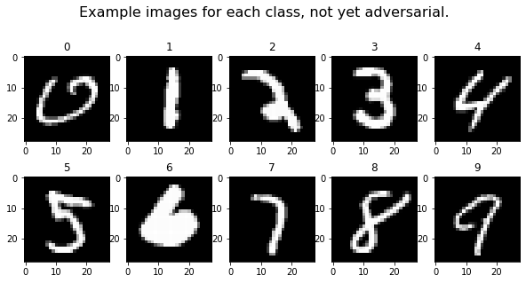
Example Images
The following ten images will be turned into adversarial samples. The images are also preprocessed, so the substitute model can accept them.
#### Code: Sample ten images
def choose_images(X, y):
    """
    Select ten random test images.
    :param X: inputs as array with shape (-1,w,h) in [0, 255]
    :param y: labels as array with shape (-1)
    :return:  test images and corresponding ground truth labels
    """
    perm = np.random.permutation(y.shape[0])
    images_for_adv = []
    y_for_adv = []

    for class_idx in range(10):
        for i, true_label in enumerate(y[perm]):
            if true_label==class_idx:
                images_for_adv.append(X[perm][i])
                y_for_adv.append(true_label)
                break

    return images_for_adv, y_for_adv

images_for_adv, y_for_adv = choose_images(x_test, y_test)
# Code: Preprocess the ten chosen images
X, y_untargeted = preprocess(np.array(images_for_adv), y_for_adv)
Plot Images
Let’s plot the ten selected images and print the oracle’s predictions. Perhaps you recall the plot_images() function from the previous parts. It is now modified to support the query_oracle() function.
# Code: Query a model on selected images and plot the results.
def plot_images(images, columns, rows, title, m=None, cmap=None):
    """
    Plot one image and the corresponding prediction per class.
    :param images:  images as numpy array with shape (-1,w,h,d) in  in [0, 1]
    :param columns: number of columns as int
    :param rows:    number of rows as int
    :param title:   title string
    :param m:       optional tensorflow.keras.Model()
    :param cmap:    optional colormap
    :note:          If no model is passed, this function will query the oracle.
    """
    fig=plt.figure(figsize=(rows*columns, columns))
    plt.suptitle(title, fontsize=16)
    for i, sample in enumerate(images):
        fig.add_subplot(rows, columns, i+1)
        # Use local model if specified. Query oracle otherwise.
        if m:
            pred = np.argmax(m.predict(sample.reshape(-1, w, h, d)))
        else:
            pred = query_oracle(back_to_image(sample))
        plt.title(pred)
        (plt.imshow(sample[...,0], cmap=cmap) if cmap else plt.imshow(sample[...,0]))
    fig.subplots_adjust(hspace=0)
    plt.show()
    return

plot_images(X, 5, 2, title="Example images for each class, not yet adversarial.", cmap="gray")
FGSM: Untargeted Attack
To the attack! This part should look familiar: You can reuse the FGSM attack class created in the white-box tutorial.
# Code: Generate adversarial samples on the ten test images
fgm_attack = FastGradientMethod(classifier=model, minimal=False, eps=0.4)
print(f"Generating {X.shape[0]} adversarial samples.")
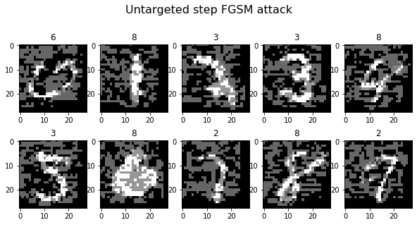
adv_x = fgm_attack.generate(x_org=X, targets=y_untargeted)
plot_images(adv_x, 5, 2, title="Untargeted step FGSM attack", cmap="gray")
Generating 10 adversarial samples.
Confusion Matrix
Those ten images only give a limited idea of our success, so let’s repeat the attack for the entire MNIST test set! That way we can observe the accuracy and confusion matrix of the attack.
# Code: Generate adversarial samples on the full MNIST test set
X_large, y_untargeted_large = preprocess(x_test, y_test)
print(f"Generating {X_large.shape[0]} adversarial samples.")
adv_x_large = fgm_attack.generate(x_org=X_large, targets=y_untargeted_large)
print(f"Querying the oracle.")
adv_y = get_oracle_predictions(back_to_image(adv_x_large))

accuracy = get_accuracy(y_test, adv_y)
print(f"Oracle accuracy after attack: {accuracy:.2f}")
print(f"Success rate of the attack: {1 - accuracy:.2f}")
plot_confusion_matrix(y_test, adv_y, title="Oracle's confusion matrix after untargeted step FGSM attack");
Generating 10000 adversarial samples.
Querying the oracle.

Oracle accuracy after attack: 0.36
Success rate of the attack: 0.64
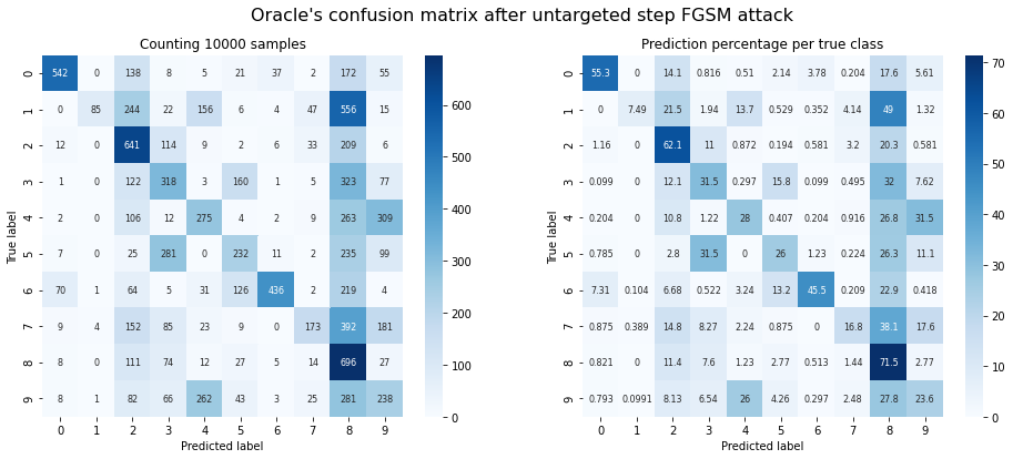
Observations: It works! There is definitely a reduction in accuracy. That said, there are a few things that stick out:
- There appears to be a tendency to create adversarial samples that are classified as ‘8’. Untargeted FGSM shifts a sample’s pixel values in the direction of the closest decision boundary. In this case a classification as ‘8’ might have the closest boundary in most cases. On the other hand, the attack utterly fails on images with ground truth class ‘8’. This indicates that other decision boundaries require more perturbation than we applied.
- For good results we must use a lot of perturbation ($\epsilon=0.4$ ). For the same untargeted FGSM attack on STL10 in the white-box tutorial $\epsilon=0.01$ was usually enough. The perturbation is so strong that the manipulation becomes obvious to an observer. This is probably also a problem with white-box attacks, though.
Let’s try to explain the need for higher perturbation: The STL10 dataset has images of size $(96, 96, 3)$ . Adversarial information can be spread across $96\times96\times3=27648$ brightness values. Compare that to MNIST with a mere $(28\times28\times1=784)$ values. There are much fewer dimensions to encode adversarial information, so the individual perturbation per pixel must be higher on MNIST.
Note: It won’t be possible to hide the perturbation with MNIST, but if an onlooker can still identify the ground truth numbers, that is an acceptable qualitative benchmark as well.
FGSM: Targeted Attack
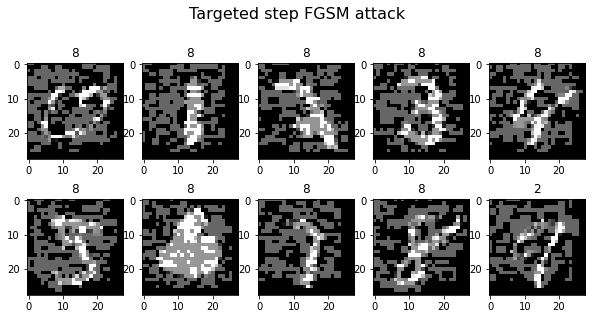
Finally, we need to create adversarial targets for the targeted attack. Remember the previous tutorials: We tried to have images of animals classified as “airplane” and technical images classified as “horse”. In this case, we’ll try to have digits below 5 classified as ‘8’ and digits larger or equal to 5 as ‘1’. If you’d like to try different targets, feel free to edit the target list.
# Code: Generate adversarial samples on the ten test images
# Define targets
target_list = [8 if i in [0, 1, 2, 3, 4,] else 1 for i in np.argmax(y_untargeted, axis=1)]
y_targeted = to_categorical(target_list, 10)

# Generate adversarial samples
fgm_attack.set_params(minimal=False, eps=0.4, targeted=True)
print(f"Generating {X.shape[0]} adversarial samples.")
adv_x = fgm_attack.generate(x_org=X, targets=y_targeted)
plot_images(adv_x, 5, 2, title="Targeted step FGSM attack", cmap="gray")
Generating 10 adversarial samples.
Confusion Matrix
# Code: Generate adversarial samples on the full MNIST test set
X_large, _ = preprocess(x_test, y_test)
target_list = [8 if i in [0, 1, 2, 3, 4,] else 1 for i in np.argmax(y_untargeted_large, axis=1)]
y_targeted_large = to_categorical(target_list, 10)

print(f"Generating {X_large.shape[0]} adversarial samples.")
adv_x_large = fgm_attack.generate(x_org=X_large, targets=y_targeted_large)
print(f"Querying the oracle.")
adv_y = get_oracle_predictions(back_to_image(adv_x_large))

print(f"Oracle accuracy after attack: {get_accuracy(y_test, adv_y):.2f}")
print(f"Success rate of the attack: {get_accuracy(adv_y, target_list):.2f}")
plot_confusion_matrix(y_test, adv_y, title="Oracle's confusion matrix after targeted step FGSM attack");
Generating 10000 adversarial samples.
Querying the oracle.

Oracle accuracy after attack: 0.12
Success rate of the attack: 0.46
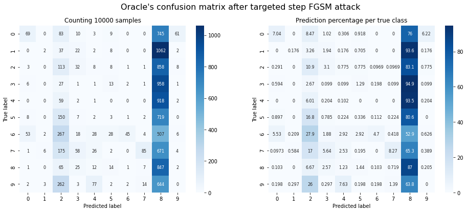
Observations: The targeted attack works only partially. This depends strongly on the target classes we choose. In this example, it is very easy to create adversarial samples classified as ‘8’, but nigh impossible to create adversarial samples classified as ‘1’.
There might be some destructive potential here: If an attacker knows which class is the easiest to achieve, they can run a targeted attack for that specific class and reduce accuracy even more than with an untargeted one.
Substitute Model: Black-Box Attack
For this attack, let’s assume the least amount of available information that you possibly can. You only know that there is some oracle that can receive images with 28x28 pixels and return predicted digits from 0 to 9.
Attacker’s Knowledge
- Unknown
- oracle architecture
- oracle parameters
- training dataset
- Known
- domain: grayscale images of digits with a resolution of $(28, 28)$
Dataset Augmentation
There is one more problem to solve: You can only query the oracle so many times. This isn’t a big deal for MNIST with its 60,000 training images - but imagine querying an oracle for a dataset the size of ImageNet. With around 150 Gigabytes worth of images, that would take a while. Even worse: Whoever is running the oracle might notice all that traffic and close down the API, block your access or implement rate limiting. Finally there’s also the point of commercial pay-per-use APIs. All things considered, you need to reduce the number of times you query the oracle.
In this case, let’s reduce the total number of queries to ~5,000. This is achieved by using a technique called Jacobian-based dataset augmentation.
Jacobian-Based Dataset Augmentation
The augmentation technique proposed by the authors works like this: Select some very small set $S_0$ of training points $\vec{x}$ . 150 random images from the MNIST test set will do. This is not enough to create a great MNIST classifier, but you only want to approximate the decision boundaries of $O$ , anyway. In other words, you want to learn the directions in which the model output is varying from those few samples.
The more input-output pairs you have, the better $F$ can approximate the decision boundaries of the oracle $O$ . To get those samples you have to create them yourself. The synthetic training points should vary in the same directions as the original 150 samples, but not be identical to them. To do this, you can take the original samples and push them further into their original direction.
You can find out the directions for each training point $\vec{x}$ by taking the Jacobian matrix of the substitute classifier $J_F$ . The directions are the sign of the Jacobian, but only for the label $\tilde{O}(\vec{x})$ returned by the oracle:
$$sgn(J_F(\vec{x})[\tilde{O}(\vec{x})]).$$To create augmented samples, this direction is added to the original samples, multiplied by a small discount value $\lambda$ :
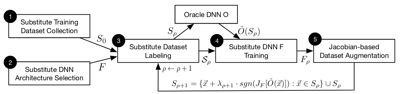
$$\vec{x}_{aug} = \vec{x} + \lambda \cdot sgn(J_F[\tilde{O}(\vec{x})])$$This is the complete training routine:
- Collect a small set $S_0$ of input data representative for the oracle’s domain.
- Select an appropriate substitute architecture.
- Query the oracle with the newly collected input data. We’ll call the labeled dataset $S_\rho$ .
- Train the substitute classifier $F$ from scratch, using data sampled from $S_\rho$ .
- Augment the input data $S_\rho$ using the Jacobian $J_F$ . This creates new data points $S_{\rho+1}$ , which include the current $S_\rho$ :
Steps 3, 4 and 5 are repeated for $\rho$ substitute training epochs.
Step 1: Collect Input Data from the Oracle’s Domain
First, take 150 images from MNIST, 15 images of each digit. They are coming from the MNIST test set, so they are images that the oracle definitely hasn’t seen before, but that fit the domain perfectly.
Alternatively, you could also create your input data by writing out the numbers yourself (the authors of the paper did it, too). Either way should work.
# Code: Create an initial dataset of 150 images.
def sample_n_of_each(X, y, n=15):
    """
    Randomly sample 10 images and ground truth labels per class from the input data.
    :param X: array of images with shape (-1,28,28)
    :param y: array of ground truth labels with shape (-1)
    :return: array X sliced to contain 10 images for each class
    :return: array y sliced to contain 10 ground truth labels for each class
    """
    index = []
    for cls in range(num_classes):
        cls_index = np.argwhere(y == cls)[:,0]
        index.append(np.random.choice(cls_index, n))
    index = np.array(index).flatten()
    return X[index], y[index]

x_sample, _ = sample_n_of_each(x_test, y_test)
Step 2: Choose an Architecture for the Substitute Model
Given that the oracle operates on image data, it is a fair assumption that a convolutional architecture should be successful. The following model architecture has been taken directly from the paper (model A). This is the same architecture used for the transferability demo.
# Code: Create substitute model graph
model = build_model_A()
# print(model.summary())
Steps 3, 4 and 5: Train Substitute Model on Limited Training Set
Dataset augmentation and substitute model training are all contained inside the class DatasetAugmentationMethod(). The method make_substitute_model() contains the actual substitute training loop. In pseudocode, this is what happens in the class object:
# Pseudocode:
# Input: (untrained) substitute model: F, oracle: O, initial samples S_0: X, training steps, discount factor: 𝜆

# Step 1: Initial collection S_0 --> X
# Step 2: Define model architecture --> F
for step in [training steps]:
    # Step 3: Query O to label samples S_ρ --> X,y
    _update_labels()
    # Step 4: Train F from scratch on X
    _train_classifier()
    # Step 5: Augment X using jacobian-based data augmentation
    _augment_samples():
        # Calculate the jacobian for every image in X
        jacobian = _jacobian(F(X))
        # Only use the derivatives that belong to the labels in y = O(X)
        jacobian = jacobian[y]
        # Apply Jacobian-based data augmentation
        X_aug = X + 𝜆 * sign(jacobian)
        # Add augmented samples to the pool
        X = X + X_aug
return F
Hyperparameters
All hyperparameters save for the batch size are taken straight from the paper.
- substitute epochs = 6
- training epochs = 5
- step size $\lambda$ = 0.01
- batch size = 10
Note: Apparently it improves performance if you switch the sign of step size lambda every couple epochs. We tried switching every two or three substitute epochs and didn’t really see a difference. But hey, it’s in the code if you want to investigate. :)
# Code: Jacobian-based dataset augmentation and training
class DatasetAugmentationMethod():
    """
    Jacobian-based data augmentation and adversarial training method. (Papernot et al. 2017).
    Paper link: https://arxiv.org/pdf/1602.02697.pdf
    :param classifier:      keras model
    :param X:               array of images to be augmented
    :param lmb:             hyperparameter step size lambda as float
    :param oracle_function: function object to encapsulate oracle query
    """

    def __init__(self, classifier, X, lmb, oracle_function):
        # Step 1: Initial collection
        self.X = X.copy()
        # Step 2: Define model architecture
        self.classifier = classifier

        self.y = np.empty([0])
        self.lmb = lmb
        self.num_classes = self.classifier.output.shape[1]
        self._oracle_function = oracle_function

    def _jacobian(self, X):
        """
        Calculate the jacobians of the classifier w.r.t. the input samples X.
        :param X: images as numpy array with shape (-1,w,h,d) in [0, 1]
        :return:  the jacobian for every input sample in X as array with shape (-1, num_classes, w, h, d)
        :note:    The batch_jacobian function is a TensorFlow operation, so a session is required.
        """
        x = self.classifier.input
        y = self.classifier.get_layer('y').output
        jacobian = batch_jacobian(y, x)
        return sess.run(jacobian, feed_dict = {self.classifier.input: X})

    def _train_classifier(self):
        """
        Train the classifier on self.X and self.y
        """
        num_epochs = 5
        batch_size = 10
        X, y = preprocess(self.X, self.y)
        tqdm_callback = TqdmCallback(verbose=0)
        history = self.classifier.fit(
            X, y,
            batch_size = batch_size,
            epochs = num_epochs,
            shuffle = True,
            callbacks = [tqdm_callback],
            verbose = 0
        )
        return

    def _augment_samples(self):
        """
        Augment samples using jacobian data augmentation
        :param X: array of images to be agumented
        :note: self.X is appended via side effect
        """
        X, _ = preprocess(self.X, self.y)
        # Calculate the jacobian for all samples X
        jacobian = self._jacobian(X)
        # Only use derivatives for the labels in y
        jacobian = np.array([jacobian[i,j] for i,j in enumerate(self.y)])
        # Apply Jacobian-based data augmentation
        X_aug = X + self.lmb * np.sign(jacobian)
        # Clip if outside of [0,1]
        X_aug = np.clip(X_aug, 0., 1.)
        # Reformat images, so they can be sent to the oracle
        X_aug = back_to_image(X_aug)
        # Add augmented samples to the pool
        self.X = np.concatenate([self.X, X_aug])
        return

    def _update_labels(self):
        """
        Updates the labels for the previously augmented samples
        """
        if np.any(self.y):
            # Label the augmented samples in dataset S_p that aren't labeled yet
            label_me = self.X[-(self.y.shape[0]):] # The latter half of self.X.
            y_aug = self._oracle_function(label_me)
            self.y = np.concatenate([self.y, y_aug])
        else:
            # Label the initial dataset S_0, if this is the first substitute epoch
            self.y = self._oracle_function(self.X)
        return

    def make_substitute_model(self):
        """
        Substitute model training loop, iteratively trains the classifier on augmented data.
        :return: the trained classifier as Keras model
        """
        steps = 6
        iter_period = 3
        for step in range(steps):
            clear_output(wait=True)
            print(f"Substitute Epoch {step+1}/{steps}\n")

            # Switch the sign of step size lambda every couple epochs.
            # Apparently this improves performance.
            if step % iter_period:
                self.lmb = self.lmb * -1.

            # Step 3: Label augmented samples by querying the oracle.
            print(f"\tStep 3: Assign labels from oracle.")
            self._update_labels()

            # Step 4: Train substitute model from scratch on augmented data (self.X ~= S_p)
            print(f"\tStep 4: Training substitute model on {self.y.shape[0]} samples.")
            sess.run(tf.initialize_all_variables())
            self._train_classifier()

            if (step+1) < steps:
                # Step 5: Augment using jacobian-based data augmentation
                print(f"\tStep 5: Augment {self.X.shape[0]} samples.")
                self._augment_samples()
            else:
                # No need to augment after the final model is trained
                print("Done.")

        return self.classifier
# Code: Train substitute model with data augmentation
sess = k.get_session()

ds_aug = DatasetAugmentationMethod(
    model,
    x_sample,
    lmb = 0.1,
    oracle_function = get_oracle_predictions
)

model = ds_aug.make_substitute_model()
Substitute Epoch 6/6

Step 3: Assign labels from oracle.

Step 4: Training substitute model on 4800 samples.

Done.
# Code: Save model to file
save_dir = os.path.join(os.getcwd(), 'saved_models')
model_name = 'model_A_black-box'
if not os.path.isdir(save_dir):
    os.makedirs(save_dir)
model_path = os.path.join(save_dir, model_name)
model.save(model_path)
# Code: Load substitute model from file
#model = load_model("saved_models/model_A_black-box")
model = load_model("final_models/model_A_black-box")
Augmentation Demo
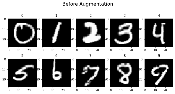
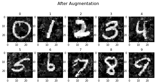
In the next two plots you can see ten un-augmented samples, followed by the same samples after six augmentation steps. It’s clearly visible that the images have been altered, but the oracle should still predict most of them correctly.
# Code: Compare augmented and unaugmented samples
demo_index = np.arange(10)*15
x_aug_proc, y_aug_proc = preprocess(ds_aug.X, ds_aug.y)
# Take 10 images from the start of the augmented dataset
plot_images(x_aug_proc[:150][demo_index], 5, 2, title="Before Augmentation", cmap="gray")
# Take 10 images from the end of the augmented dataset
plot_images(x_aug_proc[-150:][demo_index], 5, 2, title="After Augmentation", cmap="gray")
Get MNIST Performance of Substitute Model
This is just to show the prediction performance of the substitute model $F$ you just trained in comparison to the true domain of the oracle $O$ .
Note: In step 1 you sampled the initial (un-augmented) data from the MNIST test set. You shouldn’t calculate performance metrics on the MNIST test set, since that’s where the training data comes from.
print(f"MNIST train accuracy: {evaluate(model, x_train, y_train):.4f}")
60000/60000 [==============================] - 4s 64us/step
MNIST train accuracy: 0.8333
The substitute model accuracy for the black-box scenario is probably worse than the one you created for the transferability demo. This is kind of expected, since the whole training was based on only 150 training points. That doesn’t say much about the model’s ability to generate adversarial examples, though. $F$ isn’t supposed to be a good classifier. Its only job is to learn the oracle’s decision boundaries well enough to create adversarial examples.
Prepare the Attacks
Alright, your black-box substitute model is ready for action! Again, let’s reuse the FGSM white-box attack.
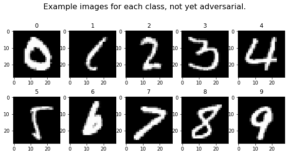
Example Images
The following ten images will be turned into adversarial samples. As with the previous attack, these images are sampled from the MNIST test set. The selected images might be part of the original training set, but don’t need to be. The images are also preprocessed, so the substitute model can accept them.
# Code: Sample ten random images
images_for_adv, y_for_adv = choose_images(x_test, y_test)
# Code: Preprocess the ten chosen images
X, y_untargeted = preprocess(np.array(images_for_adv), y_for_adv)

plot_images(X, 5, 2, title="Example images for each class, not yet adversarial.", cmap="gray")
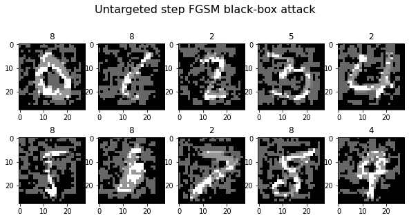
FGSM: Untargeted Attack
# Code: Generate adversarial samples on the ten test images
fgm_attack = FastGradientMethod(classifier=model, minimal=False, eps=0.4)
print(f"Generating {X.shape[0]} adversarial samples.")
adv_x = fgm_attack.generate(x_org=X, targets=y_untargeted)
plot_images(adv_x, 5, 2, title="Untargeted step FGSM black-box attack", cmap="gray")
Generating 10 adversarial samples.
Confusion Matrix
# Code: Generate adversarial samples on the full MNIST test set
X_large, y_untargeted_large = preprocess(x_test, y_test)
print(f"Generating {X_large.shape[0]} adversarial samples.")
adv_x_large = fgm_attack.generate(x_org=X_large, targets=y_untargeted_large)
print(f"Querying the oracle.")
adv_y = get_oracle_predictions(back_to_image(adv_x_large))

accuracy = get_accuracy(y_test, adv_y)
print(f"Oracle accuracy after attack: {accuracy:.2f}")
print(f"Success rate of the attack: {1 - accuracy:.2f}")
plot_confusion_matrix(y_test, adv_y, title="Oracle's confusion matrix after untargeted step FGSM black-box attack");
Generating 10000 adversarial samples.
Querying the oracle.

Oracle accuracy after attack: 0.29
Success rate of the attack: 0.71
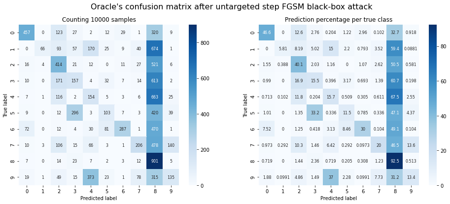
Observations: It works! Even though its own accuracy on MNIST is much worse, $F$ can create adversarial samples that fool $O$ about 70 percent of the time!
FGSM: Targeted Attack
# Code: Generate adversarial samples on the ten test images
# Define targets
target_list = [8 if i in [0, 1, 2, 3, 4,] else 1 for i in np.argmax(y_untargeted, axis=1)]
y_targeted = to_categorical(target_list, 10)
# Generate adversarial samples
fgm_attack.set_params(minimal=False, eps=0.4, targeted=True)
print(f"Generating {X.shape[0]} adversarial samples.")
adv_x = fgm_attack.generate(x_org=X, targets=y_targeted)
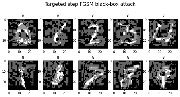
plot_images(adv_x, 5, 2, title="Targeted step FGSM black-box attack", cmap="gray")
Generating 10 adversarial samples.
Confusion Matrix
# Code: Generate adversarial samples on the full MNIST test set
X_large, _ = preprocess(x_test, y_test)
target_list = [8 if i in [0, 1, 2, 3, 4,] else 1 for i in np.argmax(y_untargeted_large, axis=1)]
y_targeted_large = to_categorical(target_list, 10)

print(f"Generating {X_large.shape[0]} adversarial samples.")
adv_x_large = fgm_attack.generate(x_org=X_large, targets=y_targeted_large)
print(f"Querying the oracle.")
adv_y = get_oracle_predictions(back_to_image(adv_x_large))

print(f"Oracle accuracy after attack: {get_accuracy(y_test, adv_y):.2f}")
print(f"Success rate of the attack: {get_accuracy(adv_y, target_list):.2f}")
plot_confusion_matrix(y_test, adv_y, title="Oracle's confusion matrix after targeted step FGSM black-box attack");
Generating 10000 adversarial samples.
Querying the oracle.

Oracle accuracy after attack: 0.18
Success rate of the attack: 0.42
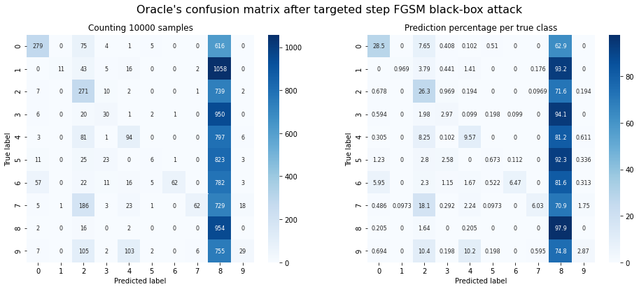
Observations: The result looks quite similar to the transferability demo, but less successful. Apparently, targeting specific decision boundaries doesn’t help much with most classes.
Note: The authors never actually describe a targeted attack, so there’s not much to compare the results against. Perhaps you’ll have more success. :)
More Black-Box Experiments
We’ve covered the Fast Gradient Sign Method in detail before. The Projected Gradient Descent Method was not converged in the substitute model paper. That said, we thought it would be handy to try at least one other way of generating adversarial samples:
PGD: Untargeted Attack
Let’s check if Projected Gradient Descent also works when using a substitute model!
# Code: Generate adversarial samples on the ten test images
pgd_attack = ProjectedGradientDescent(model, max_iter=400, eps=0.4, eps_step=0.01)
print(f"Generating {X.shape[0]} adversarial samples.")
adv_x = pgd_attack.generate(x_org=X, targets=y_untargeted)
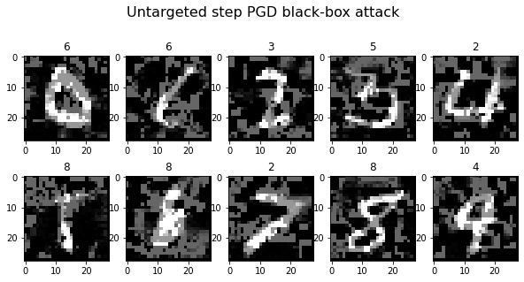
plot_images(adv_x, 5, 2, title="Untargeted step PGD black-box attack", cmap="gray")
Generating 10 adversarial samples.
Confusion Matrix
# Code: Generate and evaluate adversarial samples on the MNIST test set.
X_large, _ = preprocess(x_test, y_test)

print(f"Generating {X_large.shape[0]} adversarial samples.")
adv_x_large = pgd_attack.generate(x_org=X_large, targets=y_untargeted_large)
print(f"Querying the oracle.")
y_hat_pgd = get_oracle_predictions(back_to_image(adv_x_large))

accuracy = get_accuracy(y_test, adv_y)
print(f"Oracle accuracy after attack: {accuracy:.2f}")
print(f"Success rate of the attack: {1 - accuracy:.2f}")
plot_confusion_matrix(y_test, adv_y, title="Oracle's confusion matrix after untargeted step PGD black-box attack");
Generating 10000 adversarial samples.

Querying the oracle.

Oracle accuracy after attack: 0.18
Success rate of the attack: 0.82

Observations: The untargeted PGD attack is also successful!
- It generally manages to bring the accuracy of the oracle slightly lower than FGSM does under the same conditions.
- The attack doesn’t result in as many predictions of ‘8’ as FGSM. There are more predictions of other classes. PGD still performs worst on images with ground truth class ‘8’.
PGD: Targeted Attack
Let’s try again to have images below ‘5’ classified as ‘8’ and images starting at ‘5’ classified as 1:
# Code: Generate adversarial samples on the ten test images
pgd_attack.set_params(max_iter=400, eps=0.4, eps_step=.01, targeted=True)
print(f"Generating {X.shape[0]} adversarial samples.")
adv_x = pgd_attack.generate(x_org=X, targets=y_targeted)
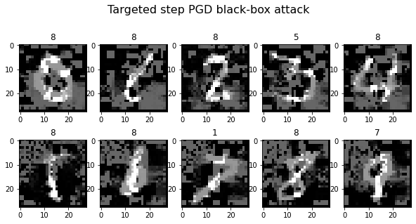
plot_images(adv_x, 5, 2, title="Targeted step PGD black-box attack", cmap="gray")
Generating 10 adversarial samples.
# Code: Generate and evaluate adversarial samples on the MNIST test set.
X_large, _ = preprocess(x_test, y_test)
target_list = [8 if i in [0, 1, 2, 3, 4,] else 1 for i in np.argmax(y_untargeted_large, axis=1)]
y_targeted_large = to_categorical(target_list, 10)

print(f"Generating {X_large.shape[0]} adversarial samples.")
adv_x_large = pgd_attack.generate(x_org=X_large, targets=y_targeted_large)
print(f"Querying the oracle.")
y_hat_pgd = get_oracle_predictions(back_to_image(adv_x_large))

# Plot results as confusion matrix.
print(f"Oracle accuracy after attack: {get_accuracy(y_test, y_hat_pgd):.2f}")
print(f"Success rate of the attack: {get_accuracy(adv_y, target_list):.2f}")
plot_confusion_matrix(y_test, y_hat_pgd, title="Oracle's confusion matrix after targeted PGD black-box attack");
Generating 10000 adversarial samples.

Querying the oracle.

Oracle accuracy after attack: 0.35
Success rate of the attack: 0.42
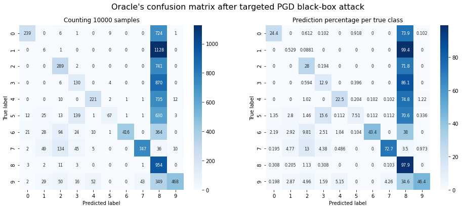
Observations: The PGD attack doesn’t fare much better on a targeted attack than FGSM did. The only difference to FGSM is that the images which it cannot turn into ‘1’, also aren’t classified as ‘8’. They are instead classified as their original class. It’s as if the PGD doesn’t quite know where to push the image.
Results Summary
If you’d like to compare your own results to ours, you can do that here:
The validation was done on the 10,000 test images of the MNIST dataset. All FGSM attacks are one-step attacks. The maximum allowed perturbation factor is $\epsilon=0.4$ for all tests. The values differ slightly across notebook executions. If everything worked and you used the same oracle model as we did, your results should look similar to this:
| Attack Method | Attack Type | Attack Success Rate (%) | Oracle Accuracy (%) |
|---|---|---|---|
| FGSM (MNIST) | untargeted | 64 | 36 |
| FGSM (black-box) | untargeted | 71 | 29 |
| PGD (black-box) | untargeted | 82 | 18 |
| FGSM (MNIST) | targeted | 46 | 12 |
| FGSM (black-box) | targeted | 42 | 18 |
| PGD (black-box) | targeted | 42 | 35 |
Final Observations
- A targeted black-box attack is often harder to achieve than an untargeted one. You can also see this with the white-box attacks from previous chapters.
- Some classes are a lot harder to force than others. For example, forcing the oracle to predict an ‘8’ is easy, while a ‘1’ is really hard. PGD fails in a different way than FGSM, but it too depends on the specific digit it’s supposed to generate.
- It is easier to change the prediction to a target that looks similar to the original. ‘4’ to ‘9’ is relatively easy, ‘0’ to ‘1’ is hard. Perhaps ‘8’ can be written in many different ways that are all similar to different digits.
- Possible explanation: In an untargeted attack, the samples are shifted towards the nearest decision boundary. In a targeted attack, the decision boundary to approach is fixed. If this boundary is very far from the current sample, the sample must be changed more drastically to be pushed in its direction. This observation should also apply to most white-box attacks.
- Most examples here require quite high $\epsilon$ values in comparison to STL10. They would likely be quite obvious to detect.
- Speculation: There are only 28x28 pixels in each MNIST image, significantly fewer than in STL10. To encode the same amount of “adversarial information” in this space, the perturbation must likely be larger per individual pixel, as it cannot be “spread over” as many dimensions.
Conclusion
On Gradient Masking
As you’ve seen, gradient masking doesn’t offer strong protection against adversarial attacks. As long as the model output is exposed to the public, it is also accessible to attackers. An adversary who can query your black-box often enough, can get enough information to build an approximation of it and attack from there.
If you find yourself in a situation where you need to defend against this type of attack, there are still some things you can do. Rate limiting may help a little: In our example attack we had to query the oracle around 5000 times. If your API only accepts one hundred queries per user and hour, that would already draw out the time required for the black-box attack from minutes to several hours. But that still doesn’t offer reliable protection if an attacker takes enough time or employs an improved technique for data augmentation, e.g. with reservoir sampling.
There are better methods to detect, filter or mitigate adversarial samples. We will explore a more recent technique in the last chapter!
Where to Look Next
- You could implement reservoir sampling. This is a technique to reduce the number of queries we must send to the oracle even more! The method is also described in the paper. [1]
- We needed to apply a bit more perturbation to achieve the same results than they did in the paper ($\epsilon = 0.4$
vs $\epsilon = 0.3$
). The authors propose using grid search on the hyperparameters they introduced. Perhaps that makes a difference. It could make sense for
- the number of substitute epochs,
- the discount value $\lambda$ ,
- the alternation rate between positive and negative $\lambda$ . [1]
- In step 4 you train your substitute model from scratch (!). For MNIST, this is totally fine. Training model $A$ for 5 epochs takes only a few seconds. If you were using a different architecture, this might be very different. That is the main reason why this chapter isn’t using an STL10-capable oracle and VGG16 (or similar) for the substitute model $F$ . At the time of writing this (mid 2020), training VGG16 on a capable GPU can easily take a week, and you would have to do that several times! Even with the reduced and augmented datasets, it could still take days to run a single substitute epoch. It should be possible to generate adversarial samples that fool a large oracle model with a much simpler substitute model.
- In black-box attacks, there are other types of information an attacker might use, outside of knowing only the data domain.[3]
- Chapter four deals with the detection of adversarial images using an autoencoder.
Other Black-Box Attacks
This is a selection. Good resources for a better overview are the 2019 survey paper [3] and IBM’s adversarial-robustness-toolbox.[4]
- ZOO: Zeroth Order Optimization Based Black-box Attack [5] A method where the attacker has access to the confidence values and can estimate the oracle’s gradients from there (More details).
- Query-Efficient Black-box Attack [6] A method where the attacker tries to reduce the number of required oracle queries. It uses evolutional strategies for sampling efficiently (More details).
Sources
[1] Practical Black-Box Attacks against Machine Learning
[2] How to Deploy your Pytorch Models with TorchServe
[3] Adversarial Attacks and Defenses in Images, Graphs and Text: A Review
[4] IBM adversarial-robustness-toolbox
[5] ZOO: Zeroth Order Optimization Based Black-box Attack
[6] Query-Efficient Black-box Attack