Institute for Applied AI

Selected Topics #1: Adversarial Attacks

Chapter 4: Countermeasure with Autoencoder Detection

This part of the tutorial explores the paper Adversarial Detection and Correction by Matching Prediction Distributions.

Contents

1. Introduction
2. Prerequisites
3. Autoencoder Training
4. Autoencoder Evaluation
5. Conclusion
6. Sources

Introduction

You have now seen several methods (white and black box) with which an attacker could cause damage. In the intro, we have already introduced you to some ways of detecting these attacks. This tutorial refers to a rather new and flexible idea, which is presented in ^[1]. The presented algorithm was introduces in February 2020 and does not need any adversarial examples to train the detector. Before you actually feed our images to our classification model $CL$ , we pass the images through an autoencoder: $AE$ .

What is an autoencoder?

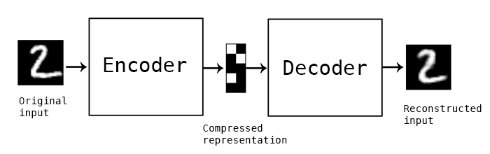
In general an autoencoder is an artificial neural network that learns how to efficiently compress and encode data and learns how to reconstruct the data back from the reduced encoded representation. There are several components:

• Encoder: The model learns how to reduce the input dimensions and compress the input data into an encoded representation.
• Bottleneck: Layer that contains the compressed representation of the input data. This is the lowest possible dimensions of the input data.
• Decoder: Model learns how to reconstruct the data from the encoded representation

Usually, autoencoders are trained to find a transformation $T$ that reconstructs the input instance $x$ as accurately as possible with loss functions that are suited to capture the similarities between x and $x'$ such as the mean squared reconstruction error.

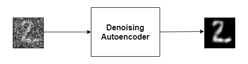
An autoencoder can perform various tasks. One area which comes very close to our needs is the Denoising Autoencoder. What do we want to achieve? In the best case we want to filter the noise out of an adversarial image so that the classification does not fail. A Denoising Autoencoder gets noisy images as input during training and is supposed to generate non-noisy images.

This could help us, but we would have to generate adversarial images during the training. This would probably only make us robust to a few specific attacks and it would take extra time. So the idea is, that we don’t consider the proximity of the two images as our loss.

Adversarial Detection and Correction by Matching Prediction Distributions ^[1]

The basic idea presented in the paper is that we remove the computation of the loss based on how close the output image is to the input image. What we more care about is that the input image and the reconstructed image should lead to the same prediction of our classification model.

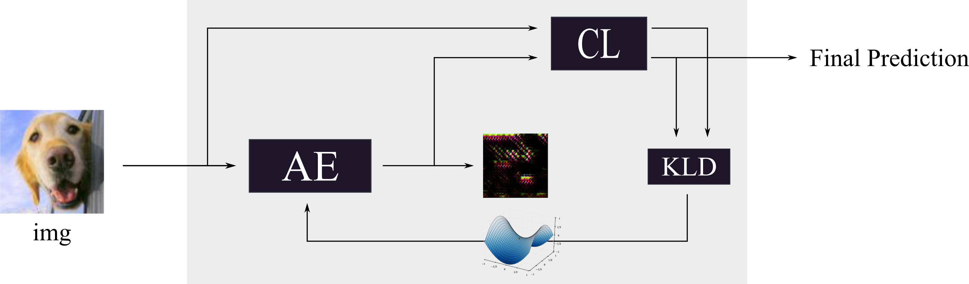
The novelty of the adversarial autoencoder (AE) detector relies on the use of a classification-model $CL$ dependent loss function based on a distance metric in the output space of the model to train the autoencoder network. Given the model $CL$ we optimize the weights of $AE$ such that the KL-divergence^[4] between the model predictions on $x$ and on $x'$ is minimized.

Without the presence of a reconstruction loss term $x'$ simply tries to make sure that the prediction probabilities $CL(x')$ and $CL(x)$ match without caring about the proximity of $x'$ to $x$ . As a result, $x'$ is allowed to live in different areas of the input feature space than $x$ with different decision boundary shapes with respect to the model $CL$ . The carefully crafted adversarial perturbation which is effective around x does not transfer to the new location of $x'$ in the feature space, and the attack is therefore neutralized. Training of the autoencoder is unsupervised since we only need access to the model prediction probabilities and the normal training instances. We do not require any knowledge about the underlying adversarial attack and the $CL$ ’s weights are frozen during training.

The underlying paper uses a threshold after the training to decide if the image is an adversarial or not. If the KL-divergence is below this threshold take the output of $CL(x)$ . In all other cases they use $CL(x')$ . This procedure is illustrated in the diagram below:

What do you implement?

• In the cell below you see a class called AE_Training. With this class you can train an autoencoder like described in the process above:

  • The autoencoder itself consists of three convolutional layer to downsample the image to the latent space (dimension=40) and three transpose convolution layer to upsample the image to the input dimension:

    ########### Downsampling path ###########
    Conv2D(32, 4)
    Conv2D(64, 4)
    Conv2D(256, 4)
    
    ########### Flatten the input to the latent space ###########
    Flatten(),
    Dense(100),
    
    ########### Upsampling path ###########
    Dense(12 * 12 * 128)
    Reshape(target_shape=(12, 12, 128))
    Conv2DTranspose(256, 4)
    Conv2DTranspose(64, 4)
    Conv2DTranspose(3, 4)
    

• This pseudo code should demonstrate the computation of the loss

  # get the output of the autoencoder
  x' = AE(x)
  
  # get the class probability distributions from the classification model from the original image
  # and the output of the autoencoder
  cl1 = CL(x')
  cl2 = CL(x)
  
  # calculate the difference of the two distribution and take it as loss
  loss = kld(cl1, cl2)
  

Prerequisites

Import modules

Below are all of the modules that must be installed and imported to run this tutorial. Use the Keras interface again to make it easier for you to understand the implementation.

import keras
from keras.models import Sequential, load_model
from keras.layers import Dense, Flatten, Conv2D, MaxPooling2D, Activation, Dropout, InputLayer, Reshape, Conv2DTranspose
import numpy as np
import os
import tensorflow as tf
from extra_keras_datasets import stl10
import keras.backend as k
from keras.applications.vgg16 import VGG16
from keras.engine import Model
from tensorflow.keras.regularizers import l1
from keras.losses import kld
import keras.backend as k
import matplotlib.pyplot as plt
from tqdm import trange

# Suppress tensorflow deprecation warnings
import tensorflow.python.util.deprecation as deprecation
deprecation._PRINT_DEPRECATION_WARNINGS = False

# import own classes and functions from .py files
from plotting import plot_images
from gradientAttack import ProjectedGradientDescent

Using TensorFlow backend.

Define classes and get data of STL10

Now you create the STL10 classes, load the data set and split the data set into test and training data.

# define the class list and preprocess data
class_list = ["airplane", "bird", "car", "cat", "deer", "dog", "horse", "monkey", "ship", "truck"]
num_classes = 10

# define width, height and dimension of images
w, h, d = 96, 96, 3

# The data, split between train and test sets:
(x_test, y_test), (x_train, y_train)= stl10.load_data()
print('x_train shape:', x_train.shape)
print(x_train.shape[0], 'train samples')
print(x_test.shape[0], 'test samples')

# Convert class vectors to binary class matrices.
# Stl10 datasets starts with class 1, not 0
y_train = keras.utils.to_categorical(y_train-1, num_classes)
y_test = keras.utils.to_categorical(y_test-1, num_classes)

# Scale data between 0 and 1
x_train = x_train.astype('float32')
x_test = x_test.astype('float32')
x_train /= 255
x_test /= 255

x_train shape: (8000, 96, 96, 3)
8000 train samples
5000 test samples

Autoencoder Training

To ensure that the weights of the classification model stay unchanged, set the trainable parameter of each layer inside the model to false. Look in the code below!

You use a latent space dimension of $100$ and train 60 epochs.

class AE_Training():
    """
    This class is used to train an autoencoder to create the same output of another model
    """

    def __init__(self, img_rows, img_cols, depth, model_cl):

        # set input dimensions
        self.img_rows = img_rows
        self.img_cols = img_cols
        self.depth = depth

        # set classification model
        self.model_cl = model_cl

        # this holds the function we used to train the model
        self.train = None

        # build the autoencoder structure
        self.model_ae =  tf.keras.Sequential(
            [
                tf.keras.layers.Conv2D(32, 4, strides=2, padding='same', input_shape = (96, 96, 3),
                       activation=tf.nn.relu, kernel_regularizer=l1(1e-5)),
                tf.keras.layers.Conv2D(64, 4, strides=2, padding='same',
                       activation=tf.nn.relu, kernel_regularizer=l1(1e-5)),
                tf.keras.layers.Conv2D(256, 4, strides=2, padding='same',
                       activation=tf.nn.relu, kernel_regularizer=l1(1e-5)),
                tf.keras.layers.Flatten(),
                tf.keras.layers.Dense(100),

                tf.keras.layers.Dense(12 * 12 * 128, activation=tf.nn.relu),
                tf.keras.layers.Reshape(target_shape=(12, 12, 128)),
                tf.keras.layers.Conv2DTranspose(256, 4, strides=2, padding='same',
                                activation=tf.nn.relu, kernel_regularizer=l1(1e-5)),
                tf.keras.layers.Conv2DTranspose(64, 4, strides=2, padding='same',
                                activation=tf.nn.relu, kernel_regularizer=l1(1e-5)),
                tf.keras.layers.Conv2DTranspose(3, 4, strides=2, padding='same',
                                activation=None, kernel_regularizer=l1(1e-5))
            ]
            )

        # set up the required operations
        self._setup_attack_graph()

        # make the layers inside the classification model not trainable
        for l in self.model_cl.layers:
            l.trainable = False


    def _setup_attack_graph(self):
        """
        Method builds up the attack graph
        """

        ### Placeholder for the input images
        x = k.placeholder(dtype=tf.float32, shape = (None, self.img_rows, self.img_cols, self.depth))

        # Feed the image through the autoencoder
        x_pred = self.model_ae(x)

        # let the classification model predict the output of ae and original input
        cl1 = self.model_cl(x_pred)
        cl2 = self.model_cl(x)

        # calculate kld loss
        loss_function = tf.keras.losses.kld
        loss_kld = loss_function(cl1, cl2)
        loss = tf.reduce_mean(loss_kld)

        # optimizer
        opt = tf.keras.optimizers.Adam(learning_rate=0.001)
        # we only want to update the parameters of the ae model
        updates = opt.get_updates(loss, self.model_ae.trainable_weights)

        # create a keras function
        self.train = k.function([x],
                                [loss], updates=updates)


    def fit(self, x_train):
        """
        Method trains the autoencoder
        :param x_train    Training Images
        """
        print("Start training of AE...")

        # initialize the variables of the autoencoder model
        k.get_session().run(tf.variables_initializer(self.model_ae.trainable_weights))

        # define hyperparameters
        epochs = 60
        batch_size  = 128
        no_batches = int(np.ceil(len(x_train)/batch_size))

        # create dataset to iterate over
        dataset = tf.data.Dataset.from_tensor_slices(x_train).shuffle(1024).batch(batch_size).repeat(epochs)
        iterator = tf.data.make_one_shot_iterator(dataset)
        next_batch = iterator.get_next()

        last_loss = np.Inf
        # train the model for n_epochs
        for i in range(epochs):
            losses = []
            for batch in range(no_batches):
                train_batch = k.get_session().run(next_batch)
                losses.append(self.train([train_batch]))
            print(f"Epoch {i} -----> avg. batch loss: {np.mean(losses)}")

            if np.mean(losses) < last_loss:
                print("Save model")
                # save the model
                self.model_ae.save("../final_models/autoencoder_60_100.h5")
                last_loss = np.mean(losses)

Do Training and save the model

classification_model = load_model("./final_models/vgg16_stl10.h5")
ae = AE_Training(96, 96, 3, classification_model)
ae.fit(x_train)

Autoencoder Evaluation

Step 1: Loading the models

First you need to load our models. We load the trained autoencoder, which should remove the noise from our adversarial examples and our white box model, which we want to protect with the autoencoder module, is the fine tuned VGG16 model.

How to create a white-box model? Have look here: Creating your white box model

autoencoder = tf.keras.models.load_model("./final_models/autoencoder_60_100.h5")
classification_model = load_model("./final_models/vgg16_stl10.h5")

Step 2: Validate Autoencoder with the test dataset

Now check the accuracy of $CL$ on the test dataset. Then pass all test data through $AE$ and check the output of $CL$ .

print(f"Accuracy of CL without AE : {classification_model.evaluate(x_test, y_test)[1]}")

5000/5000 [==============================] - 5s 937us/step
Accuracy of CL without AE : 0.7874000072479248

print(f"Accuracy of CL on AE's output : {classification_model.evaluate(autoencoder.predict(x_test), y_test)[1]}")

5000/5000 [==============================] - 3s 555us/step
Accuracy of CL on AE's output : 0.5569999814033508

Observations:

You can see that the AE is not able to learn good representations for all images. This could certainly be improved by fine-tuning, but it is not so important for our use case to achieve a high accuracy. It is more relevant to consider the difference in accuracy between adversarial and non-adversarial.

Plot some examples

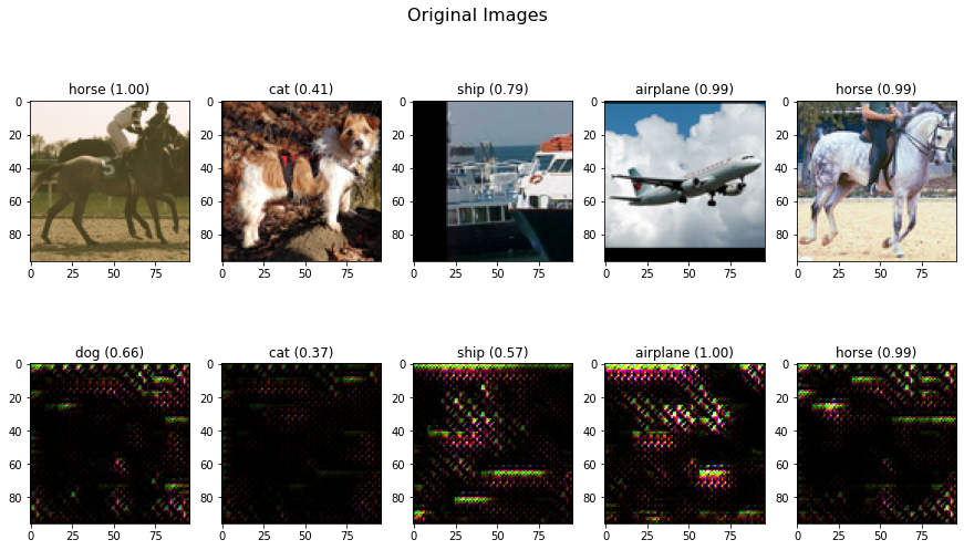
Now you can view a few examples to see the differences between the learned image of the autoencoder and the original image,

org_images = x_test[50:55]
ae_images = autoencoder.predict(x_test[50:55])
plot_imgs = np.array([org_images, ae_images]).reshape(-1, w, h, d)

# this function is imported from a python file. It's the same like in the GradientAttack tutorial
plot_images(plot_imgs, 5, 2, title="Original Images", model=classification_model, ae=True)

Observations:

You have three cases here:

• the ship, airplane and the horse to the right are well classified by $CL$ on the original images and also on the $AE$ ’s output
• the horse to the left is predicted correct by the $CL$ , but after the $AE$ the prediction is dog. So the transformation during the training leads to some loss of information here
• The autoencoder is able to reconstruct an image which leads to the same false prediction of the dog.

Attack Images on classification model

In addition to the original images, you also have created some attack images with the presented PGD method. You have saved the images and read them in in the cell below.

First you validate the attack images, by looking at the performance of our white box model.

attack_images = []
gt = []
for path in os.listdir("./detector_data/imgs/attack/"):
    img = plt.imread("./detector_data/imgs/attack/" + path)
    gt.append(path.split(".")[0])
    attack_images.append(img/255.)
attack_images = np.array(attack_images)

plot_images(attack_images, 5, 2, title="Attack Images on CL", model=classification_model, gt=gt)

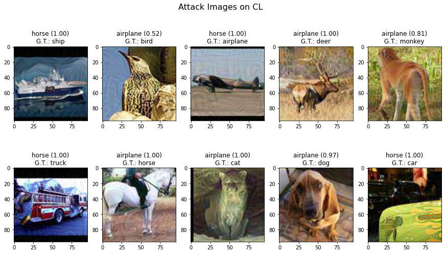
You see that the targeted attack is successful for almost every image. Only the bird is not classified as airplane

Attack Images on classification model after AE

Let’s test, if our autoencoder can remove the adversarial noise.

You first feed the attack images to the autoencoder and then use its output at input for the vgg network.

attack_pred_ae = autoencoder.predict(attack_images)
plot_images(attack_pred_ae, 5, 2, title="Attack Images on CL after AE", model=classification_model, gt=gt, ae=True)

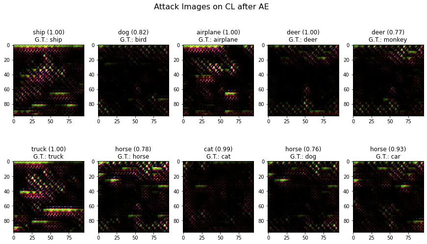
For more than half of the images you can successfully remove the adversarial perturbation and achieve the correct prediction. As described, you might need to fine tune the autoencoder to increase its performance.

Step 3: Validate the Autoencoder with all test data

Accuracy on test data without attack

This gives us the baseline performance of the VGG network on the test images

acc_org = classification_model.evaluate(x_test, y_test, batch_size=64)
print(f"Accuracy on orginal images: {acc_org[1]:.2f}")

5000/5000 [==============================] - 3s 642us/step
Accuracy on orginal images: 0.79

Do Attack on all test images

You now use the ProjectedGradientDescent class you have presented in the previous tutorial to create adversarial images for all 5000 test images. You use a untargeted attack.

Because of memory issues, we cannot create adversarial images of all images in one step. Therefore split the test images in batches of 500 and concat the results afterwards. This should be familiar to you:

# attack on all test images
pgd_attack = ProjectedGradientDescent(classification_model, max_iter=10, eps=0.03, eps_step=0.001)
adv_all = []

for i in range(0, (len(x_test)-500)+1, 500):
    print(f"Image indices from {i} to {i+500}")
    adv_x = pgd_attack.generate(x_org=x_test[i:i+500], targets=y_test[i:i+500])
    adv_all.append(adv_x)

adv_all = np.array(adv_all).reshape(-1, w, h, d)

Image indices from 0 to 500

Image indices from 500 to 1000

Image indices from 1000 to 1500

Image indices from 1500 to 2000

Image indices from 2000 to 2500

Image indices from 2500 to 3000

Image indices from 3000 to 3500

Image indices from 3500 to 4000

Image indices from 4000 to 4500

Image indices from 4500 to 5000

Accuracy on test data with attack

Let’s see the effect of the attack images by looking at the accuracy of the VGG model on the adversarial images

print(f"Accuracy of CL on attack images: {classification_model.evaluate(adv_all, y_test)[1]}")

5000/5000 [==============================] - 3s 564us/step
Accuracy of CL on attack images: 0.07800000160932541

Almost all 5000 images are falsely classified! You have an accuracy close to zero.

Accuracy on test data with attack after AE

Again, you use the autoencoder first and run the classification model afterwards

print(f"Accuracy of CL on attack images after AE: {classification_model.evaluate(autoencoder.predict(adv_all), y_test)[1]}")

5000/5000 [==============================] - 3s 557us/step
Accuracy of CL on attack images after AE: 0.5497999787330627

You get almost 55% accuracy if you use the autoencoder before the classification model. This is very close to the baseline. That means, for that images, where the autoencoder is able to reconstruct an image that gives as the same output of the $CL$ as an original image, the noise can be removed successfully.

Conclusion

We find that the Matching Prediction Distribution approach works quite well on our Adversarials and an exciting countermeasure strategy has been found here. We improve our adversarial examples from 0% accuracy to 55%. The overall accuracy is not so important at this point, but rather the difference between the autoencoder-accuracies of adversarial and non-adversarial images. Here we don’t see any differences and each reaches 55%. This means that the autoencoder is able to remove perturbation in almost all images for which it has achieved a similar probability distribution of the classification model compared to the raw input. This value can certainly be improved by fine-tuning the autoencoder. You could change the whole architecture, add new layer, remove layers, change the hyperparameters of each layer or of the training. So there are many degrees of freedom you can still experiment with. Based on our investigations, we have come to the conclusion that the approach of using an autoencoder as a detector works. Since we do not use adversaries in training, we are also very flexible regarding different types of noise and adversarial attacks and can train the autoencoder easily.The extent to which the model also achieves success on images from other attack types must be investigated further.

Where to Look Next

Now you are at the end of the tutorial. We summarize all chapters in the Introduction-notebook and give you ideas for further tutorials.

Sources

[1] Adversarial Detection and Correction by Matching Prediction Distributions
[2] Autoencoders in Keras
[3] Denoising autoencoders
[4] KL-divergence